


文章目录
A 二维曲线
A.a plot

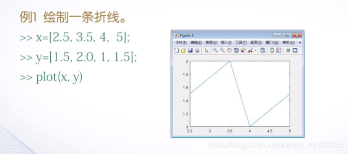
例子:
>>  x = [2.5,3.5,4,5];
>>  y = [1.5,2.0,1,1.5];
>>  plot(x,y)
>> x = [1.5,2,1,1.5];
>> plot(x)
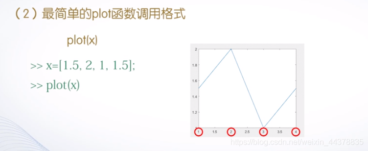
图形的横坐标,是x元素的索引
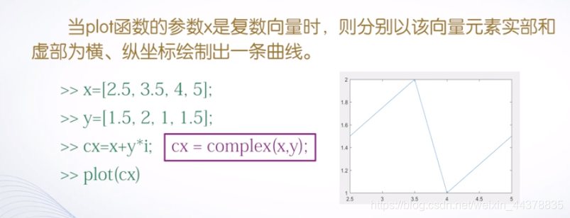
>>  x = [2.5,3.5,4,5];
>>  y = [1.5,2,1,1.5];
>> cx = x + y*i;
>> plot(cx)

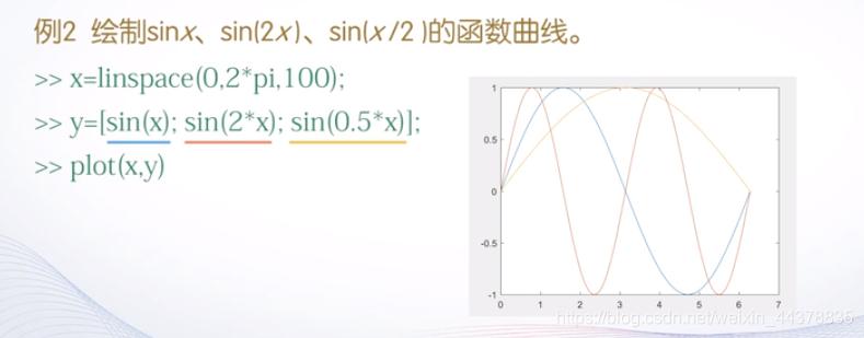
例子:
>> x = linspace(1,2*pi,100);
>> y = [sin(x);sin(2*x);sin(0.5*x)];
>> plot(x,y);
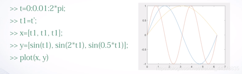
>> t = 0:0.01:2*pi;
%t1为t的转置 为列向量
>> t1 = t';
>> x = [t1,t1,t1];
>> y = [sin(t1),sin(2*t1),sin(0.5*t1)];
>> plot(x,y)


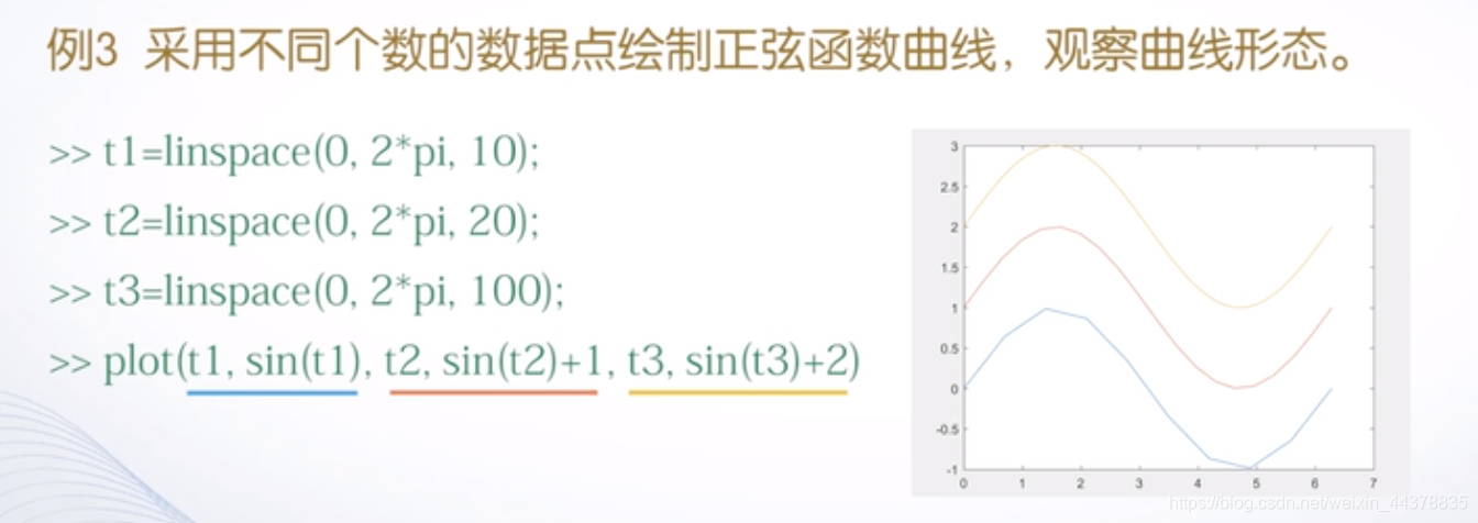
例子:
>> t1 = linspace(0,2*pi,10);
>> t2 = linspace(0,2*pi,20);
>> t3 = linspace(0,2*pi,100);
>> plot(t1,sin(t1),t2,sin(t2)+1,t3,sin(t3)+2)
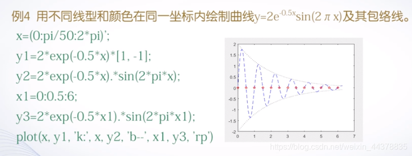
例子:
>> x = (0:pi/50:2*pi)';
%两个包络线
>> y1 = 2*exp(-0.5*x)*[1,-1];
>> y2 = 2*exp(-0.5*x).*sin(2*pi*x);
>> x1 = 0:0.5:6;
>> y3 = 2*exp(-0.5*x1).*sin(2*pi*x1);
%‘k:’黑色虚线包络线 ‘b--’蓝色双画线 ‘rp’红色五角星
>> plot(x,y1,'k:',x,y2,'b--',x1,y3,'rp')
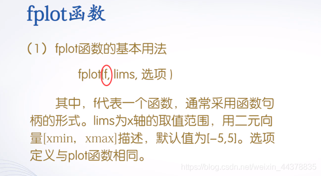
A.b fplot
x往往采取等间隔采样,如果在函数随着自变量的变化未知或者在不同区间的函数频率特性差别大,如果采用plot函数时自变量的采样间隔设置不合理,则无法反映函数的变化趋势。例如:
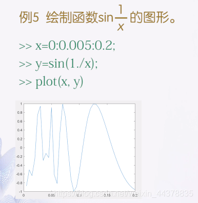
如何解决这个问题呢?——fplot可根据参数函数的变化特性,自适应地设置采样间隔。
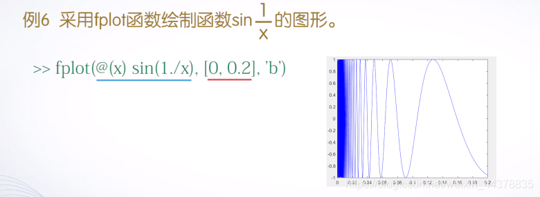
例子:
>> fplot(@(x)sin(1./x),[0,0.2],'b')

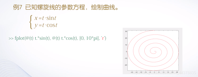
例子:
>> fplot(@(t)t.*sin(t),@(t)t.*cos(t),[0,10*pi],'r')
B 绘制图形的辅助操作
B.a 给图形添加标注

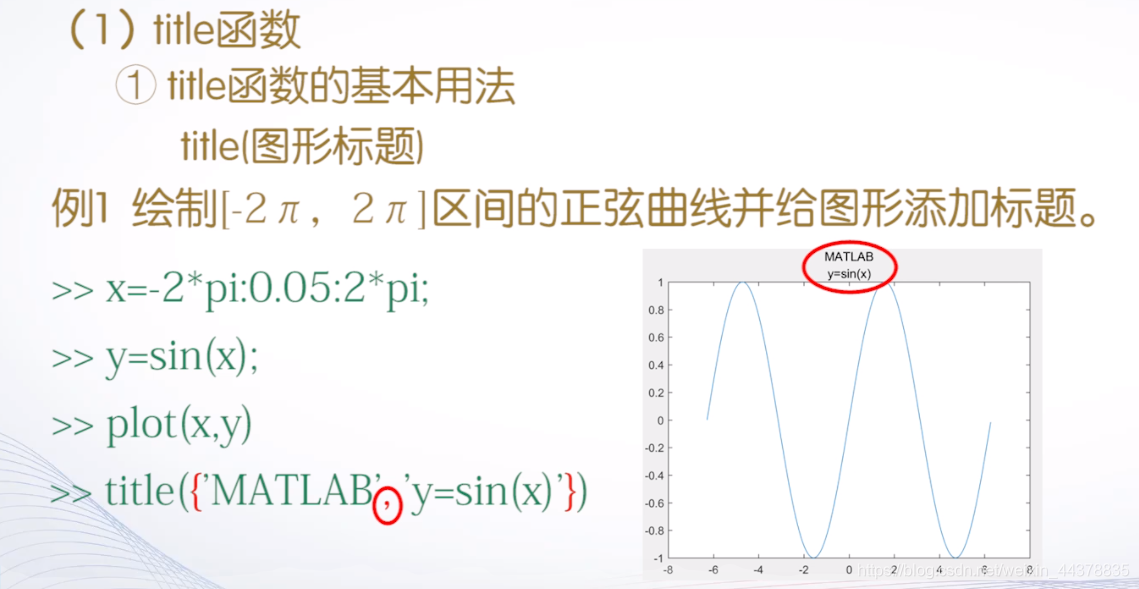
B.a.a title函数
x = -2*pi:0.05:2*pi;
y = sin(x);
plot(x,y)
title('y = sin(x)')
>> x = -2*pi:0.05:2*pi;
y = sin(x);
plot(x,y)
title({'MATLAB','y = sin(x)'})
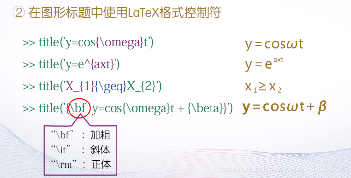
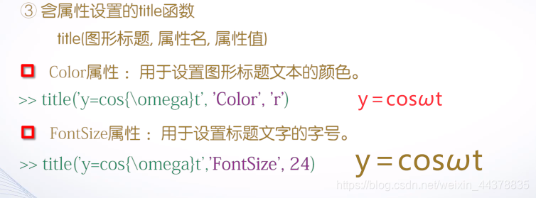
>> title(' y = cos{\omega}t')
>> title('y = e^{axt}')
>> title('X_{1}{\geq}X_{2}')
>> title('{\bf y = cos{\omega}t+{\beta}}')

颜色默认黑色
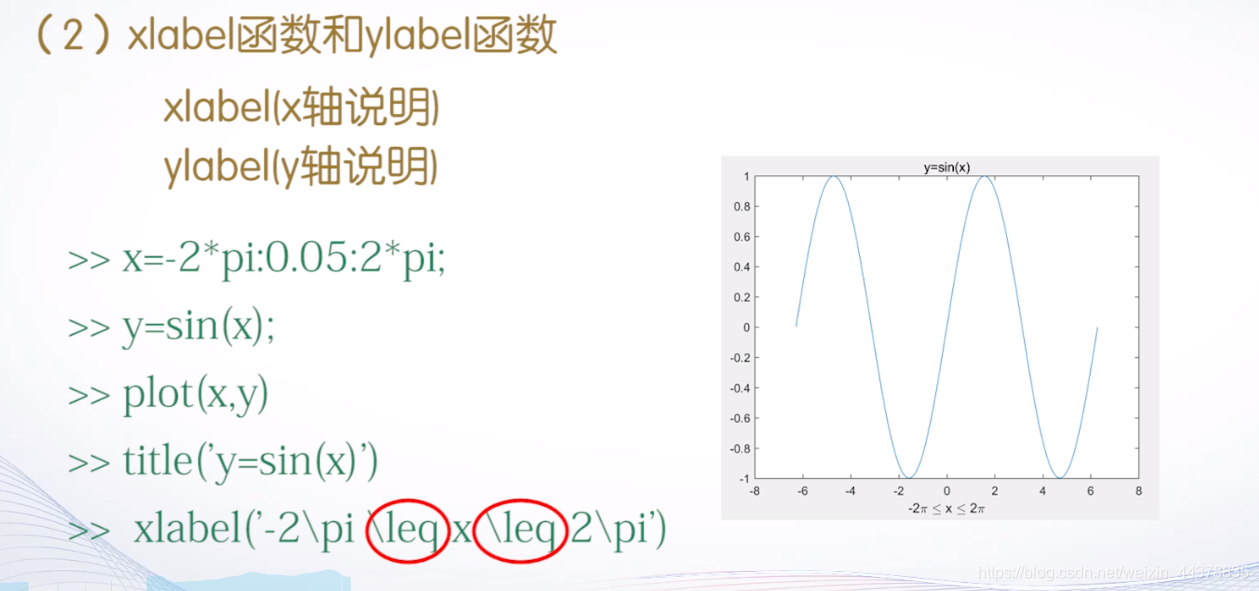
B.a.b xlabel函数和ylabel函数
x = -2*pi:0.05:2*pi;
y = sin(x);
plot(x,y)
title('y = sin(x)')
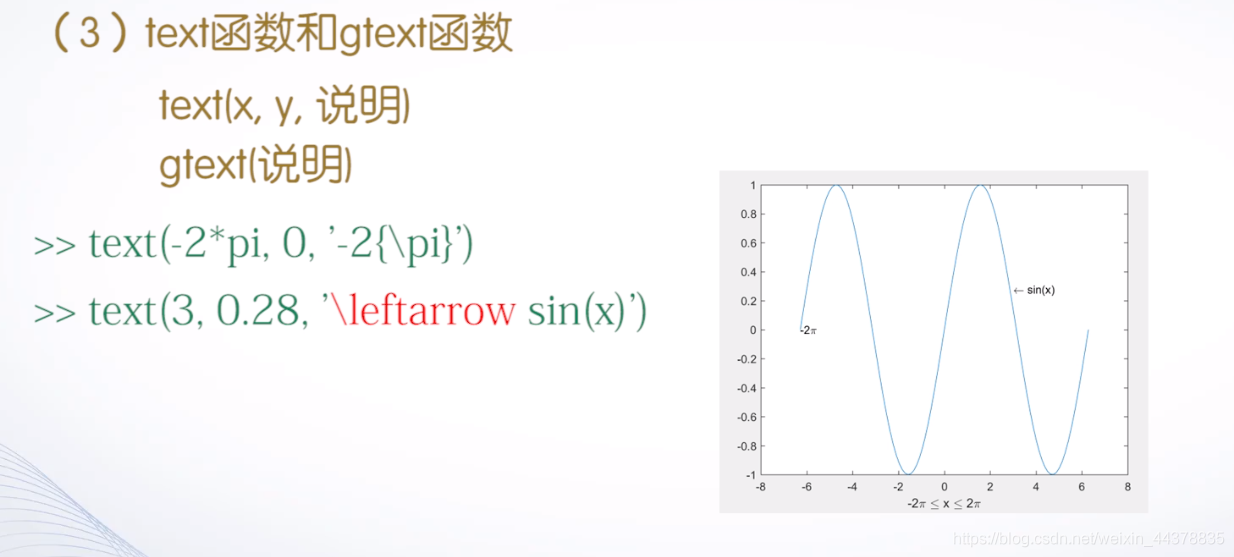
xlabel('-2\pi\leqx\leq2\pi')
text(-2*pi,0,'-2{\pi}')
text(3,0.28,'\leftarrow sin(x)')
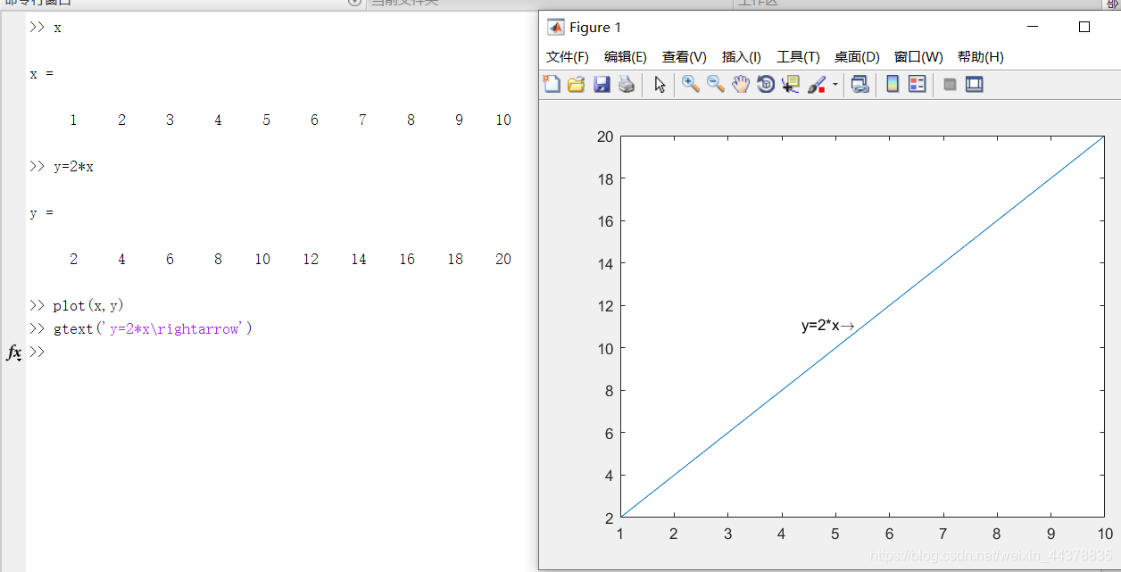
B.a.c text函数和gtext函数
gtext 函数没有参数
鼠标移动单击即可添加
gtext函数没有坐标参数,执行命令时,十字光标跟随鼠标移动,单击鼠标,即可将说明放置在十字光标处。
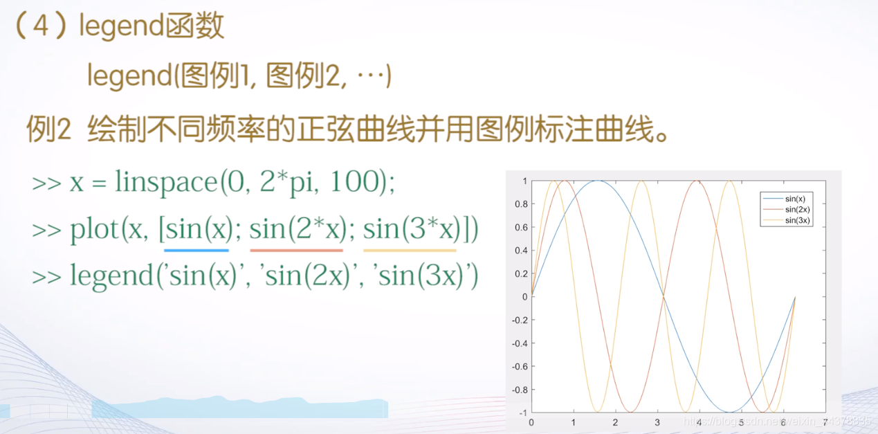
B.a.d legend函数
x = linspace(0,2*pi,100);
plot(x,[sin(x);sin(2*x);sin(3*x)])
legend('sin(x)','sin(2x)','sin(3
B.b 坐标控制
B.b.a axis函数
例子:
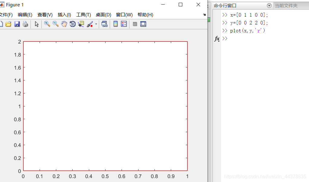
x = [0,1,1,0,0];
y = [0,0,1,1,0];
plot(x,y)
axis([-0.1,1.1,-0.1,1.1])
axis equal;

例子:
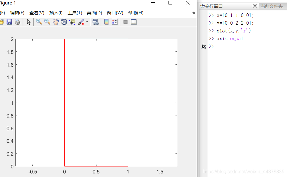
axis equal后,如:x轴0到1长度等于y轴0到1长度。消除因为x轴和y轴刻度长不等带来的图像变形。
ps:整个过程图形没有关闭。
B.b.b 给坐标系加网格和边框(grid)

grid on:控制显示网格线
grid off:控制不显示网格线
grid:在两种状态之间进行切换

用法同grid
例题:
 x = linspace(0,2*pi,100);
 y = [sin(x);sin(2*x);sin(0.5*x)];
 plot(x,y)
 %指定坐标轴刻度范围
 axis([0,7,-1.2,1.2])
 title('不同频率正弦函数曲线');
 xlabel('Variable X');
 ylabel('Variable Y');
 %显示每一条曲线对应的计算公式
 text(2.5,sin(2.5),'sin(x)');
 text(1.5,sin(2*1.5),'sin(2x)');
 text(5.5,sin(0.5*5.5),'sin(0.5x)');
 legend('sin(x)','sin(2x)','sin(0.5x)')
 grid on
B.c 图形保持(hold)
在已经存在的图形叠加图形
hold on   % 控制保持原有图形
hold off  % 控制刷新图形窗口
hold      % 两种模式间切换
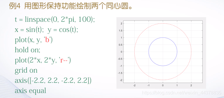
例子:
t = linspace(0,2*pi,100);
x = sin(t);
y = cos(t);
plot(x,y,'b')
hold on;
plot(2*x,2*y,'r--')
grid on
axis([-2.2,2.2,-2.2,2.2])
axis equal
B.d 图形窗口的分割(subplot)

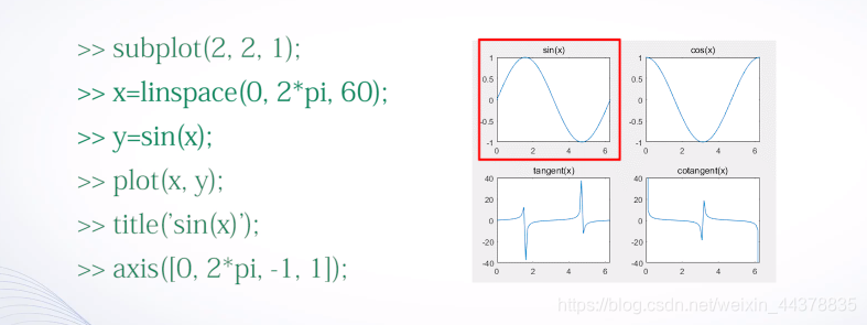
例子(显示一个子图的代码):
subplot(2,2,1);
x = linspace(0,2*pi,60);
y = sin(x);
plot(x,y);
title('sin(x)');
axis([0,2*pi,-1,1]);
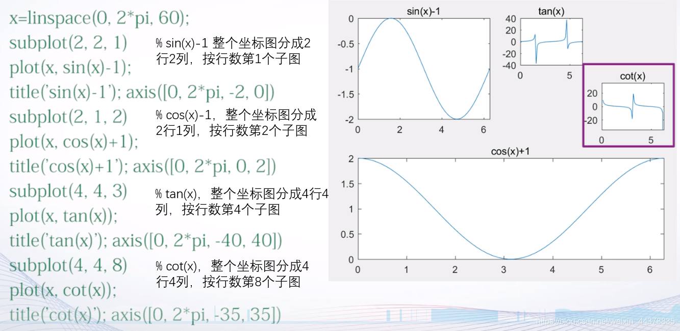
例子:
x = linspace(0,2*pi,60);
subplot(2,2,1);
plot(x,sin(x)-1);
title('sin(x)-1');
axis([0,2*pi,-2,0])
subplot(2,1,2);
plot(x,cos(x)+1);
title('cos(x)+1');
axis([0,2*pi,0,2])
subplot(4,4,3);
plot(x,tan(x));
title('tan(x)');
axis([0,2*pi,-40,40])
subplot(4,4,8);
plot(x,cot(x));
title('cot(x)');
axis([0,2*pi,-35,35]);
C 其他形式的二维图形
C.a 其他坐标系下的二维曲线图
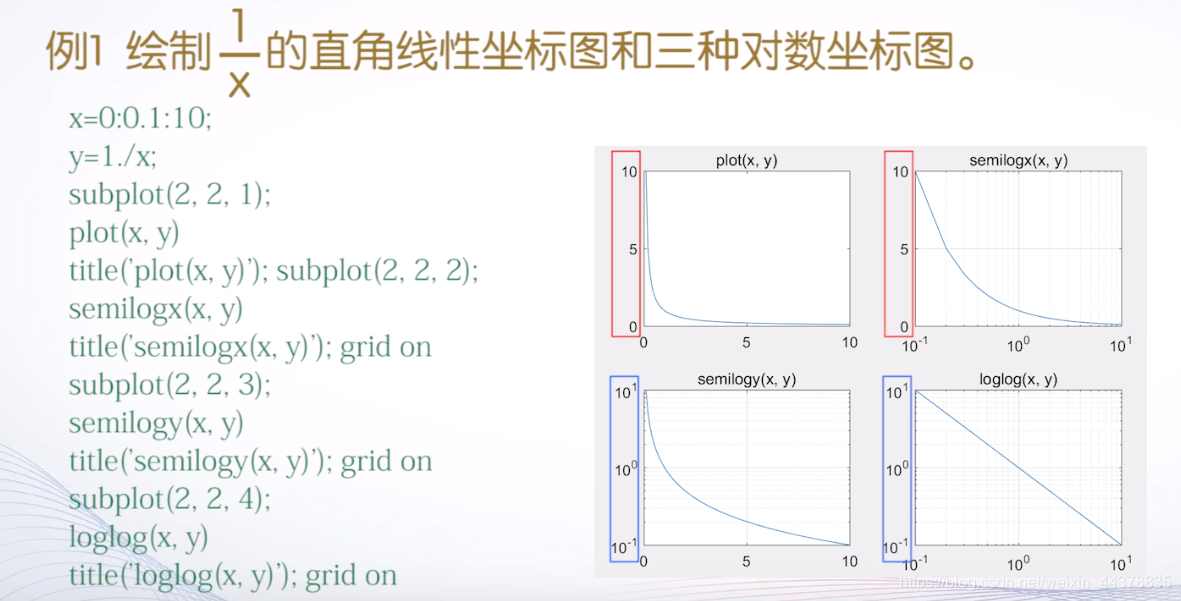
C.a.a 对数坐标图(semilogx;semilogy;loglog)

semilogx: x使用常用对数刻度,y为线性刻度
semilogy: y使用常用对数刻度,x为线性刻度
loglog:x,y都使用常用对数刻度
例子:
x = 0:0.1:10;
y = 1./x;
subplot(2,2,1);
plot(x,y)
title('plot(x,y)');
subplot(2,2,2);
semilogx(x,y)
title('semilogx(x,y)');
grid on
subplot(2,2,3);
semilogy(x,y)
title('semilogy(x,y)');
grid on
subplot(2,2,4);
loglog(x,y)
title('loglog(x,y)');
grid on
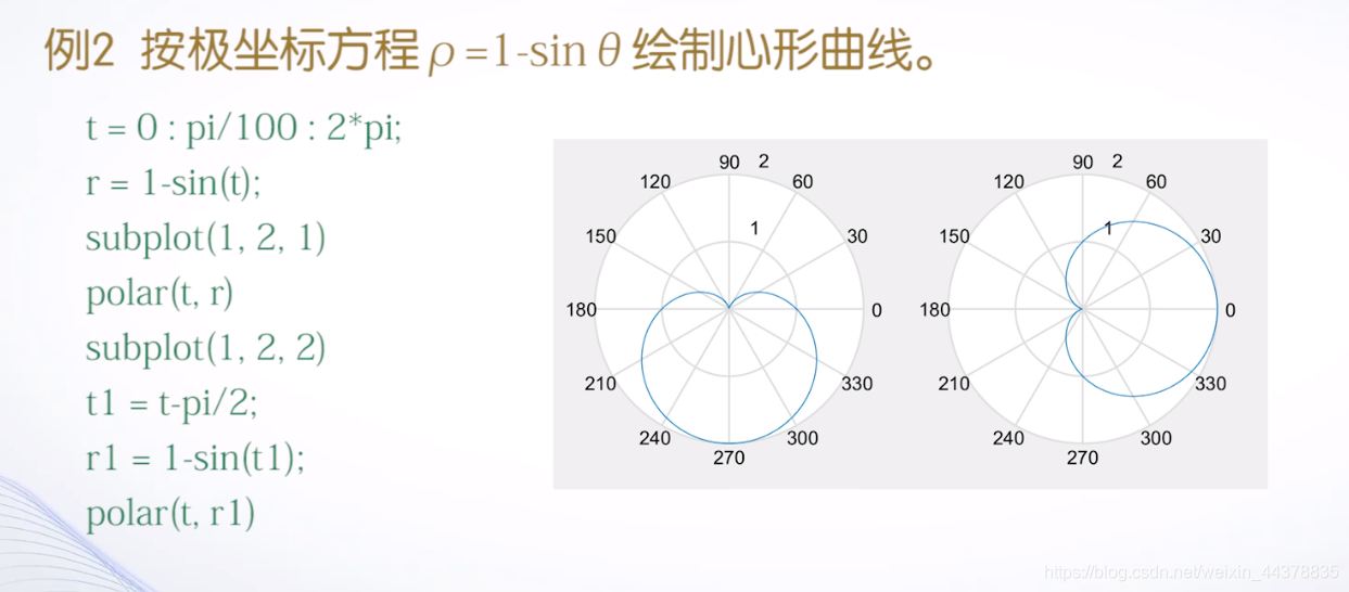
C.a.b 极坐标图(polar)
t = 0: pi/100:2*pi;
r = 1-sin(t);
subplot(1,2,1)
polar(t,r)
subplot(1,2,2)
t1 = t-pi/2;
r1 = 1-sin(t1);
polar(

C.b 统计图
C.b.a 条形类图形(bar、barh;hist、rose)

bar:竖直条形图
barh:水平条形图

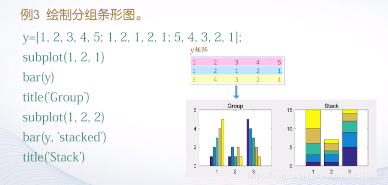
例子:
y = [1,2,3,4,5;1,2,1,2,1;5,4,3,2,1];
subplot(1,2,1);
bar(y);
title('Group');
subplot(1,2,2)
bar(y,'stacked');
title('Stack')

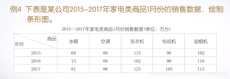
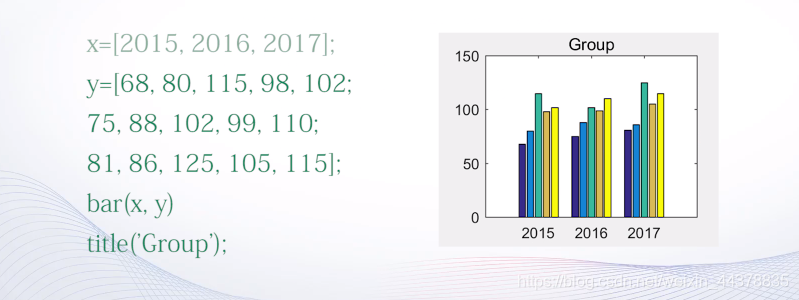
例题:
x = [2015,2016,2017];
y = [68,80,115,98,102;
    75,88,102,99,110;
    81,86,125,105,115];
bar(x,y)
title('Group');

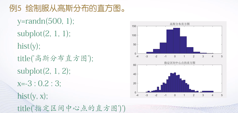
hist:直角坐标系
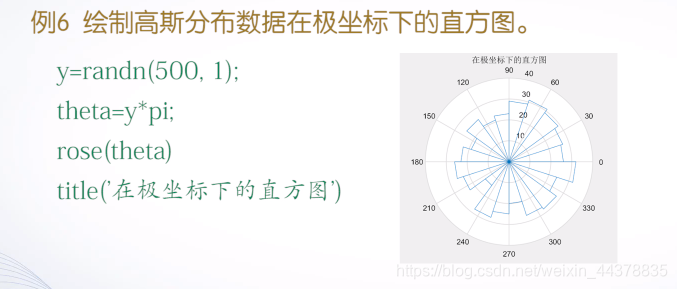
rose:极坐标系

x:用于设置统计区间的划分方式,若统计数据为标量,则统计数据均分为x个小区间,若x是向量,则x中的每一个数指定分组的中心值,元素的个数为数据分组数,x缺省时,默认按10个等分区间进行统计。
y = randn(500,1);
subplot(2,1,1);
hist(y);
title('高斯分布直方图');
subplot(2,1,2);
x = -3:0.2:3;
hist(y,x);
title('指定区间中心点的直

theta:是一个向量,绘图时将圆划分为若干个角度相等的扇形区域,每个扇形高度为落入这个扇形区域的theta个数。如果x是标量,则将0到2pi划分为x个扇形区域,默认20。
例子:
C.b.b 面积类图形(pie;area)

例子:
score = [5,17,23,9,4];
ex = [0,0,0,0,1];
pie(score,ex);
%location 位置 eastouside右边外侧
%如果无指定 会遮挡图形
legend('优秀','良好','中等','及格','不及格','location','eastoutside')

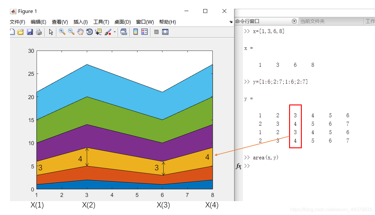
area(x, y):该函数以参数x和y绘制面积图。如果x和y为向量,则相当于函数plot(x, y),并将0到y之间进行了填充。如果参数y为矩阵,则将y的每一列绘制面积图并进行叠加。
例子:
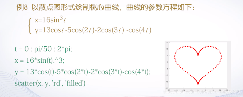
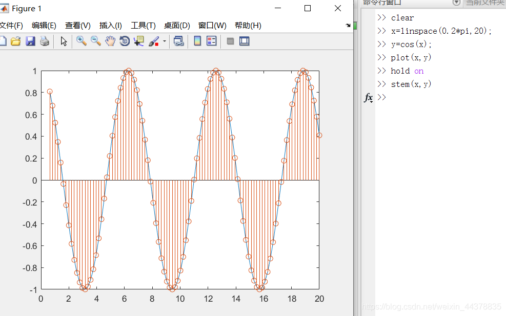
C.b.c 散点类图形(scatter;stairs;stem)
用法与plot类似。


filed:填充数据点标记
例子:
t = 0:pi/50:2*pi;
x = 16*sin(t).^3;
y = 13*cos(t)-5*cos(2*t)-2*cos(3*t)-cos(4*t);
%filled数据点实心
scatter(x,y,'rd','filled');
stairs:

stem:
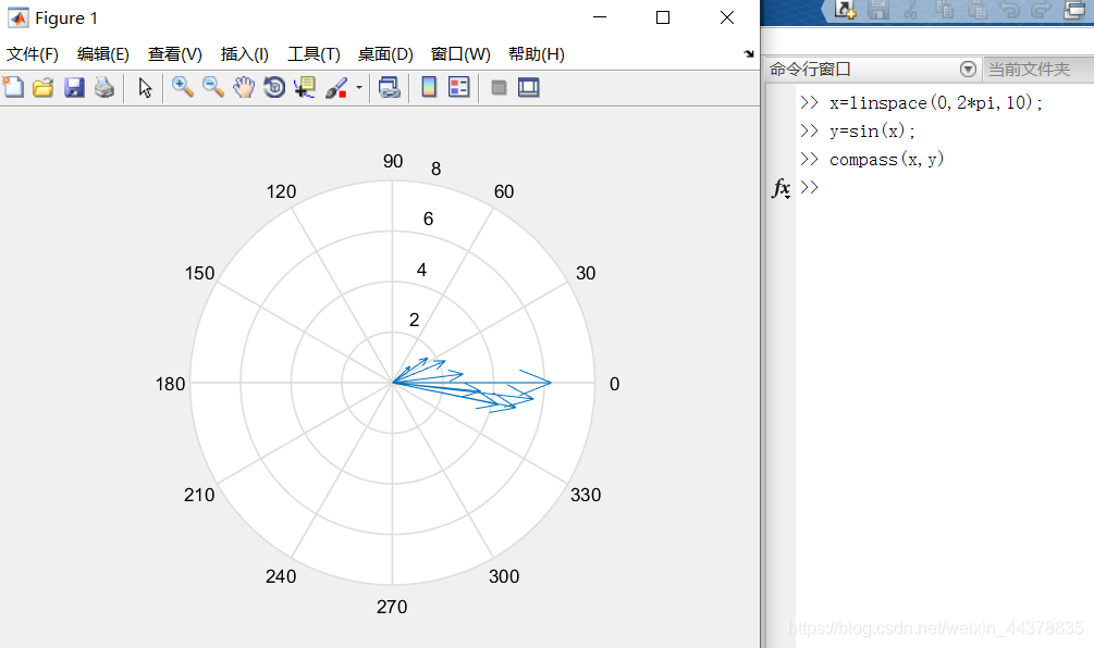
C.c 矢量图形(compass;feather;quiver)

compass:
compass(x,y):x,y是n维向量,显示n个箭头,箭头的起点为原点,箭头位置为(x(i),y(i)).
compazz(z):参量z为n维复数向量,命令显示n个箭头,箭头起点为原点,箭头位置为(real(z),image(z))。
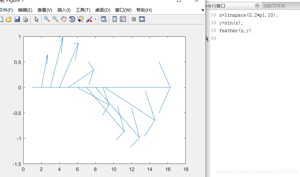
feather:
feather(x,y) :函数绘制由向量参量x与y构成的速度向量,沿水平轴方向,从均匀间隔点以箭头发射出来;’
feather(z) :函数绘制羽毛图。参量z是一个复数,则feather(z)相当于compass(real(z),imag(z));

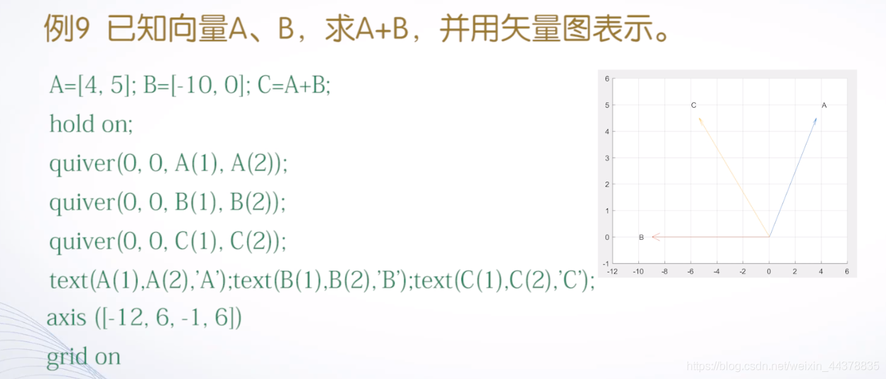
例子:
A = [4,5];
B = [-10,0];
C = A+B;
hold on;
quiver(0,0,A(1),A(2));
quiver(0,0,B(1),B(2));
quiver(0,0,C(1),C(2));
%三点进行标注
text(A(1),A(2),'A');
text(B(1),B(2),'B');
text(C(1),C(2),'C');
axis([-12,6,-1,6]);
grid on
部分图片来源:
https://www.icourse163.org/search.htm?search=%E4%B8%AD%E5%8D%97%E5%A4%A7%E5%AD%A6%20Matlab#/


 1029
1029


 被折叠的 条评论
为什么被折叠?
被折叠的 条评论
为什么被折叠?
 到【灌水乐园】发言


