Python 基于sklearn （1）- 数据预处理-构建好的训练数据集

本文数据预处理主要步骤：

（1）删除和估算缺失值 （removing and imputing missing values）

（2）获取分类数据 （Getting  categorical data into shape for machine learning）

（3）为模型构建选择相关特征 （Selecting relevant features for the module construction）

【创建CSV数据集】

[python]  view plain  copy

1. #build a csv dataset   
2. import numpy as np  
3. import pandas as pd  
4. from io import StringIO  
5. import sys  
6. #数据不要打空格，IO流会读入空格  
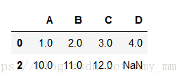
7. csv_data = \  
8. '''''A,B,C,D 
9. 1.0,2.0,3.0,4.0 
10. 5.0,6.0,,8.0 
11. 10.0,11.0,12.0, 
12. '''  
13. df = pd.read_csv(StringIO(csv_data))  

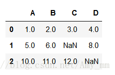
如图，有两个空值~

【统计空值情况】

[python]  view plain  copy

1. #using isnull() function to check NaN value   
2. df.isnull().sum()  

【访问数组元素】

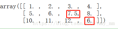
在放入sklearn的预估器之前，可以通过value属性访问numpy数组的底层数据

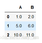
【消除缺失值 dropna() 函数】

一个最简单的处理缺失值的方法就是直接删掉相关的特征值（一列数据）或者相关的样本（一行数据）。

利用dropna()函数实现。

dropna( axis = 0 /1 )参数axis表示轴选择，axis=0 代表行，axis=1 代表列。

[python]  view plain  copy

1. df.dropna(axis = 1)  

[python]  view plain  copy

1. df.dropna(axis = 0)  

dropna( how = all) how参数选择删除行列数据（any / all）

df.dropna(how = 'all')

dropna(thresh = int) 删除值少于int个数的值

[python]  view plain  copy

1. df.dropna(thresh = 4)  

dropna( subset = [' '])  删除指定列中有空值的一行数据（整个样本）

[python]  view plain  copy

1. df.dropna(subset = ['C'])  

删除C列中有空值的那一行数据

虽然直接删除很是简单啦~但是天下没有免费的午餐，直接删除会带来很多弊端。比如样本值删除太多导致不能进行可靠预测；或者特征值删除太多（列数据），可能失去很多有价值的信息。

所以下面介绍一个更为通用的缺失值处理技巧——插值技术。我们可以根据样本集中的其他数据，运用不同的插值技术，来估计 样本的缺失值。

【插值】interpolation techniques

【imputing missing values】

比较常用的一种估值是平均值估计（mean imputation）。可以直接使用sklearn库中的imputer类实现。

[python]  view plain  copy

1. <span style="font-size:16px;">class sklearn.preprocessing .Imputer</span>  

[python]  view plain  copy

1. <span style="font-size:16px;">(missing_values = 'NaN', strategy = 'mean', axis = 0, verbose = 0, copy = True)</span>  

参考：http://scikit-learn.org/stable/modules/generated/sklearn.preprocessing.Imputer.html

参数说明：

missing_values : int或者'NaN',默认NaN（string类型）

strategy：默认mean。平均值填补。

可选项： mean（平均值）

              median（中位数）

              most_frequent（众数）

axis： 指定轴向。axis= 0，列向（默认）；axis= 1，行向。

verbose : int 默认值为0

copy：默认True,创建数据集的副本。

          False:在任何合适的地方都可能进行插值。

以下四种情况，即使copy设为False,也会进行创建副本：

                    1. X不是浮点型数组

                    2.X是稀疏矩阵，且missing_values= 0

                    3.axis=0,X被编码为CSR矩阵（Compressed Sparse Row 行压缩）

                    4.axis=1，X被编码为CSC矩阵（Copressed Sparse Column 列压缩）

[python]  view plain  copy

1. #mean imputation  
2. #axis = 0,表示列向，采用每一列的平均值填补空值  
3.   
4. from sklearn.preprocessing import Imputer  
5. imr = Imputer(missing_values = 'NaN', strategy = 'mean', axis = 0 )  
6. imr = imr.fit(df.values)  
7. imputed_data = imr.transform(df.values)  
8. imputed_data  

【处理分类数据】

handling categorical data

分类数据一般分为nominal（名词性，不可排序）和ordinal（可排序数据）

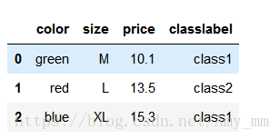
 【创建分类数据集】

[python]  view plain  copy

1. #create categorical dataset   
2. import pandas as pd  
3. df = pd.DataFrame([  
4.     ['green', 'M', 10.1, 'class1'],  
5.     ['red', 'L', 13.5, 'class2'],  
6.     ['blue', 'XL', 15.3, 'class1']  
7. ])  
8. df.columns = ['color', 'size', 'price', 'classlabel']  
9. df  

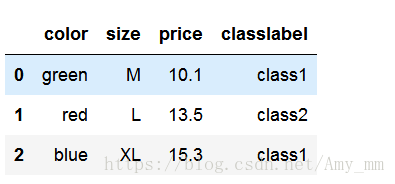
nominal data : color

ordinal data : size

numerical data : price

 【映射可排序特征】

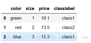
为确保学习算法能够正确识别可排序特征值，需要将分类数据转换为数值型数据。

[python]  view plain  copy

1. #converting categorical string values into integers  
2. size_mapping = {  
3.     'XL': 3,  
4.     'L' : 2,  
5.     'M' : 1}  
6. df['size'] = df['size'].map(size_mapping)  
7. df  

也可以反向映射回分类值

[python]  view plain  copy

1. #reverse mapping   
2. inv_size_mapping = {  
3.     v : k for k ,v in size_mapping.items()  
4. }  
5. df['size'] = df['size'].map(inv_size_mapping)  
6. df  

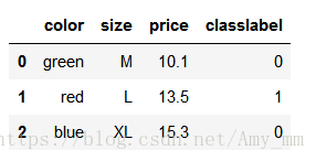
【编码分类标签】

Encoding class label

[python]  view plain  copy

1. import numpy as n  
2. class_mapping = {label : idx for idx, label in enumerate(np.unique(df['classlabel']))}  
3. class_mapping  

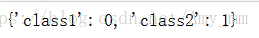
利用上述class_mapping将classlabel转换为integer

[python]  view plain  copy

1. df['classlabel'] = df['classlabel'].map(class_mapping)  
2. df  

同样可以转换回去

[python]  view plain  copy

1. inv_class_mapping = {v : k for k, v in class_mapping.items()}  
2. df['classlabel'] = df['classlabel'].map(inv_class_mapping)  
3. df  

也可以直接调用sklearn库中的LabelEncoder 类进行类标签转换

[python]  view plain  copy

1. #直接采用sklearn库中的LabelEncoder进行编码  
2. from sklearn.preprocessing import LabelEncoder  
3. class_le = LabelEncoder()  
4. y = class_le.fit_transform(df['classlabel'].values)  
5. y  

利用inverse_transform转换回去

[python]  view plain  copy

1. class_le.inverse_transform(y)  

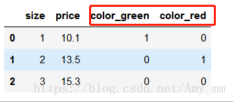
【one-hot encoding for nominal features】

get_doommies()

使用one-hot编码时，容易引起共线性问题，在使用其他算法时容易出现bug,例如矩阵的求逆。

为避免这种问题，降低变量间的相关性，可以简单的删除one-hot编码数组中特征值的第一列，这样也不会丢失重要信息。

例如删除color_blue这一列，如果color_red=0,color_green=0,则可以判断color_blue=1.

[python]  view plain  copy

1. pd.get_dummies(df[['size','color','price']],drop_first = True)  

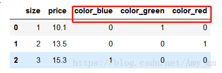
删除color_blue这一列，令drop_firt=True即可

[python]  view plain  copy

1. #为避免共线性问题，降低变量间的相关性，删除one-hot数组中特征值的第一列  
2. pd.get_dummies(df[['size','color','price']],drop_first = True)  

【数据特征选择】

利用wine dataset 学习特征选择，以及L1，L2Z正则化数据。

【读数据】

[python]  view plain  copy

1. # read wine dataset  
2. df_wine = pd.read_csv("G:\Machine Learning\python machine learning\python machine learning code\code\ch04\wine.data")  
3. df_wine.columns = ['Class label', 'Alcohol', 'Malic acid', 'Ash',  
4.                    'Alcalinity of ash', 'Magnesium', 'Total phenols',  
5.                    'Flavanoids', 'Nonflavanoid phenols', 'Proanthocyanins',  
6.                    'Color intensity', 'Hue', 'OD280/OD315 of diluted wines',  
7.                    'Proline']  
8.   
9. print('Class labels', np.unique(df_wine['Class label']))  
10. df_wine.head()  

【划分数据 ——训练集和测试集】

[python]  view plain  copy

1. #seperate train and test data  
2. from sklearn.model_selection import train_test_split  
3. X,y = df_wine.iloc[:,1:].values,df_wine.iloc[:,0].values  
4. X_train, X_test, y_train, y_test = \  
5.                 train_test_split(X,   
6.                                  y,   
7.                                  test_size = 0.3,   
8.                                  random_state = 0,   
9.                                  stratify = y)  

【feature scaling】

特征缩放在数据预处理中是及其重要的一步，除了决策树和随机森林中不需要特征缩放，其余大部分学习和优化算法都需要特征缩放，保证所有特征在同一范围内。

两个进行特征缩放的方法：normalization（规范化） and standardization（标准化）

对比两种放缩的实例数据：

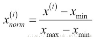
Normalization:将数据重新规范到范围[0,1]之间，是min-max缩放中的一种。

计算公式：

 sklearn.preprocessing.MinMaxScaler 实现

1. #sklearn normalization  
2. from sklearn.preprocessing import MinMaxScaler  
3. mms = MinMaxScaler()  
4. X_train_norm = mms.fit_transform(X_train)  
5. X_test_norm = mms.transform(X_test)  

Standardization:将数据标准化为均值为0 方差为1

计算公式：

 

1. sklearn standardization  
2. from sklearn.preprocessing import StandardScaler  
3. stdsc = StandardScaler()  
4. X_train_std = stdsc.fit_transform(X_train)  
5. X_test_std = stdsc.transform(X_test)  

只需要在训练集上使用fit函数，然后使用这些参数去标准化测试集或者其他新的数据集。这样就可以使得所有标准化后的数据在同一scale上，是课相互比较的数据集。

【避免过拟合的方法】

（1）收集尽可能多的训练数据

（2）通过正则化引入对于模型负责度的惩罚系数

（3）选择参数较少的简单模型

（4）降级数据维度

方法（1）一般不太可行

本文讲述通过特征选择实现的正则化和降低纬度的方法使得模型简单化。

【L1 L2正则化】

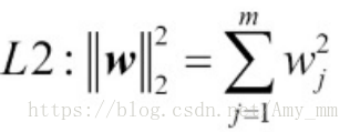
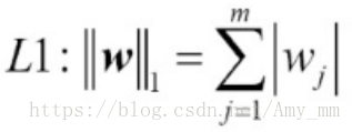
L1正则化通常会生成稀疏特征向量，大部分特征值为0。

如果数据集是高维度且有很多不相关的特征值，尤其是当不相关的维度多于样本时，L1是很好的选择。

sklearn 实现L1 L2

[python]  view plain  copy

1. # sklearn实现L1  
2. from sklearn.linear_model import LogisticRegression  
3. lr = LogisticRegression(penalty = 'l1', C = 1.0)  
4. lr.fit(X_train_std,y_train)  
5. print('Training accuracy:', lr.score(X_train_std, y_train))  

SBS（Sequential Backward Selection） 序列后向选择

从特征全集开始，每次从特征集中删除一个特征x，使得删除特征x后评价函数值达到最优。

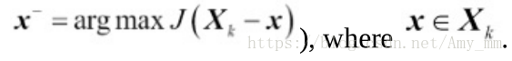
算法：定义一个判别函数J，目的是是J最小化

（1）初始化 k=d,d是数据集的维数

（2）选择使得判别函数最大的特征,

（3）从特征集中删除特征

（4）如果k达到了期望值，结束；否则返回（2）

[python]  view plain  copy

1. <span style="font-weight:normal;">#SBS select features  
2. from sklearn.base import clone  
3. from itertools import combinations  
4. import numpy as np  
5. from sklearn.metrics import accuracy_score  
6. from sklearn.model_selection import train_test_split  
7. class SBS():  
8.     def __init__(self,   
9.                  estimator, #评估器 比如LR，KNN  
10.                  k_features, #想要的特征个数  
11.                  scoring = accuracy_score,#对模型的预测评分  
12.                  test_size=0.25,   
13.                  random_state=1):  
14.           
15.         self.scoring = scoring  
16.         self.estimator = clone(estimator)  
17.         self.k_features = k_features  
18.         self.test_size = test_size  
19.         self.random_state = random_state  
20.           
21.     def fit(self, X, y):  
22.         #seperete train data and test data  
23.         X_train, X_test, y_train, y_test = train_test_split(X, y,   
24.                                                             test_size = self.test_size,   
25.                                                             random_state = self.random_state)  
26.         # dimension   
27.         dim = X_train.shape[1]  
28.         self.indices_ = tuple(range(dim))  
29.         self.subsets_ = [self.indices_] #特征子集  
30.         score = self._calc_score(X_train, y_train, X_test, y_test, self.indices_)  
31.         self.scores_ = [score]  
32.           
33.           
34.         while dim > self.k_features:  
35.             scores = [] #分数  
36.             subsets = [] #子集  
37.               
38.             for p in combinations(self.indices_, r = dim - 1):  
39.                   
40.                 score = self._calc_score(X_train,  
41.                                          y_train,  
42.                                          X_test,  
43.                                          y_test,  
44.                                          p)  
45.                   
46.                 print(p, score)   
47.                   
48.                 scores.append(score)  
49.                 subsets.append(p)  
50.               
51.             best = np.argmax(scores)  
52.             self.indices_ = subsets[best]  
53.             self.subsets_.append(self.indices_)  
54.             dim -= 1  
55.               
56.             self.scores_.append(scores[best])  
57.         self.k_score_ = self.scores_[-1]  
58.         return self  
59.       
60.     def transform(self, X):  
61.         return X[:, self.indices_]  
62.   
63.     def _calc_score(self, X_train, y_train, X_test, y_test, indices):  
64.         self.estimator.fit(X_train[:, indices], y_train)  
65.         y_pred = self.estimator.predict(X_test[:, indices])  
66.         score = self.scoring(y_test, y_pred)  
67.         return score  
68. </span>  

[python]  view plain  copy

1. <span style="font-weight:normal;">import matplotlib.pyplot as plt  
2. from sklearn.neighbors import KNeighborsClassifier  
3.   
4. knn = KNeighborsClassifier(n_neighbors=5)  
5.   
6. # selecting features  
7. sbs = SBS(knn, k_features=1)  
8. sbs.fit(X_train_std, y_train)  
9.   
10. # plotting performance of feature subsets  
11. k_feat = [len(k) for k in sbs.subsets_]  
12.   
13. plt.plot(k_feat, sbs.scores_, marker='o')  
14. plt.ylim([0.7, 1.02])  
15. plt.ylabel('Accuracy')  
16. plt.xlabel('Number of features')  
17. plt.grid()  
18. plt.tight_layout()  
19. # plt.savefig('images/04_08.png', dpi=300)  
20. plt.show()</span>  

【随机森林评估特征值的重要性】

[python]  view plain  copy

1. <span style="font-weight:normal;">#随机森林选择特征值  
2. from sklearn.ensemble import RandomForestClassifier  
3.   
4. feat_labels = df_wine.columns[1:]  
5. forest = RandomForestClassifier(n_estimators=500, random_state=1)  
6.   
7. forest.fit(X_train, y_train)  
8. #  
9. importances = forest.feature_importances_  
10.   
11. indices = np.argsort(importances)[::-1]  
12.   
13. for f in range(X_train.shape[1]):  
14.     print("%2d) %-*s %f" % (f + 1, 30,   
15.                             feat_labels[indices[f]],   
16.                             importances[indices[f]]))  
17.   
18. plt.title('Feature Importance')  
19. plt.bar(range(X_train.shape[1]),   
20.         importances[indices],  
21.         align='center')  
22.   
23. plt.xticks(range(X_train.shape[1]),   
24.            feat_labels[indices], rotation=90)  
25. plt.xlim([-1, X_train.shape[1]])  
26. plt.tight_layout()  
27. plt.show()  
28. </span>  

【SelectFromModel 实现特征提取】

[python]  view plain  copy

1. <span style="font-weight:normal;">#SelectFromModel  
2. </span>from sklearn.feature_selection import SelectFromModel<span style="font-weight:normal;">  
3. sfm = SelectFromModel(forest, threshold = 0.1, prefit = True) #threshold阈值  
4. X_selected = sfm.transform(X_train)  
5. print('Number of samples that meet this criterion:',X_selected.shape[0]</span>  

[python]  view plain  copy

1. <span style="font-weight:normal;">for f in range(X_selected.shape[1]):  
2.     print("%2d) %-*s %f" % (f + 1, 30,                  #%-*s ，其中*表示输出string间隔  
3.                             feat_labels[indices[f]],   
4.                             importances[indices[f]]))</span>