


目录
选做题:使用pytorch实现Convolution Demo
5.2卷积神经网络的基础算子
卷积神经网络是目前计算机视觉中使用最普遍的模型结构,如图5.8 所示,由M个卷积层和b个汇聚层组合作用在输入图片上,在网络的最后通常会加入K个全连接层。

从上图可以看出,卷积网络是由多个基础的算子组合而成。下面我们先实现卷积网络的两个基础算子:卷积层算子和汇聚层算子。
5.2.1卷积算子
卷积层是指用卷积操作来实现神经网络中一层。为了提取不同种类的特征,通常会使用多个卷积核一起进行特征提取。
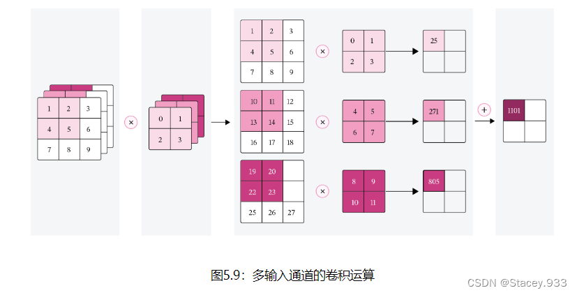
5.2.1.1多通道卷积
在前面介绍的二维卷积运算中,卷积的输入数据是二维矩阵。但实际应用中,一幅大小为的图片中的每个像素特征表示的不仅仅只有灰度值的标量,通常有多个特征,可以表示为
维的向量,比如RGB三个通道的特征向量。因此,图像上的卷积操作的输入数据通常是一个三维张量,分别对应了图片的高度
,宽度
和深度
,其中深度
通常也被称为输入通道数
。如果输入的是灰度图像,则输入通道数为1;如果输入是彩色图像,分别有
、
、
三个通道,则输入通道数为3。
此外 ,由于具有单个核的卷积每次只能提取一种类型的特征,即输出一张大小为的特征图(Feature Map)。而在实际应用中,我们也希望每一个卷积层能够提取多种不同类型的特征,所以一个卷积层通常会组合多个不同的卷积核来提取特征,经过卷积运算后会输出多张特征图,不同的特征图对应不同类型的特征。输出特征图的个数通常将其称为输出通道数
。
说明:
《神经网络与深度学习》将Feature Map翻译为“特征映射”,这里翻译为“特征图”。
假设一个卷积层的输入特征图,其中
为特征图的尺寸,
代表通道数;卷积核为
,其中
为卷积核的尺寸,
代表输入通道数,
代表输出通道数。
在实践中,根据目前深度学习框架中张量的组织和运算性质,这里特征图的大小为,和《神经网络与深度学习》中
的定义并不一致。
相应地,卷积核WW的大小为。
一张输出特征图的计算

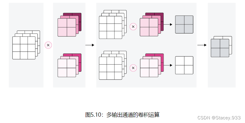
多张输出特征图的计算
对于大小为的输入特征图,每一个输出特征图都需要一组大小为
的卷积核进行卷积运算。使用
组卷积核分布进行卷积运算,得到
个输出特征图
。然后将
个输出特征图进行拼接,获得大小为
的多通道输出特征图。上面计算方式的可视化如下图5.10所示。
5.2.1.2多通道卷积层算子
根据上面的公式,多通道卷积卷积层的代码实现如下:
import torch
import torch.nn as nn
class Conv2D(nn.Module):
def __init__(self, in_channels, out_channels, kernel_size, stride=1, padding=0,weight_attr=[],bias_attr=[]):
super(Conv2D, self).__init__()
# 创建卷积核
weight_attr = torch.randn([out_channels, in_channels, kernel_size,kernel_size])
weight_attr = torch.nn.init.constant(torch.tensor(weight_attr,dtype=torch.float32),val=1.0)
self.weight = torch.nn.Parameter(weight_attr)
# 创建偏置
bias_attr = torch.zeros([out_channels, 1])
bias_attr = torch.tensor(bias_attr,dtype=torch.float32)
self.bias = torch.nn.Parameter(bias_attr)
self.stride = stride
self.padding = padding
# 输入通道数
self.in_channels = in_channels
# 输出通道数
self.out_channels = out_channels
# 基础卷积运算
def single_forward(self, X, weight):
# 零填充
new_X = torch.zeros([X.shape[0], X.shape[1]+2*self.padding, X.shape[2]+2*self.padding])
new_X[:, self.padding:X.shape[1]+self.padding, self.padding:X.shape[2]+self.padding] = X
u, v = weight.shape
output_w = (new_X.shape[1] - u) // self.stride + 1
output_h = (new_X.shape[2] - v) // self.stride + 1
output = torch.zeros([X.shape[0], output_w, output_h])
for i in range(0, output.shape[1]):
for j in range(0, output.shape[2]):
output[:, i, j] = torch.sum(
new_X[:, self.stride*i:self.stride*i+u, self.stride*j:self.stride*j+v]*weight,
[1,2])
return output
def forward(self, inputs):
"""
输入:
- inputs:输入矩阵,shape=[B, D, M, N]
- weights:P组二维卷积核,shape=[P, D, U, V]
- bias:P个偏置,shape=[P, 1]
"""
feature_maps = []
# 进行多次多输入通道卷积运算
p=0
for w, b in zip(self.weight, self.bias): # P个(w,b),每次计算一个特征图Zp
multi_outs = []
# 循环计算每个输入特征图对应的卷积结果
for i in range(self.in_channels):
single = self.single_forward(inputs[:,i,:,:], w[i])
multi_outs.append(single)
# print("Conv2D in_channels:",self.in_channels,"i:",i,"single:",single.shape)
# 将所有卷积结果相加
feature_map = torch.sum(torch.stack(multi_outs), 0) + b #Zp
feature_maps.append(feature_map)
# print("Conv2D out_channels:",self.out_channels, "p:",p,"feature_map:",feature_map.shape)
p+=1
# 将所有Zp进行堆叠
out = torch.stack(feature_maps, 1)
return out
inputs = torch.tensor([[[[0.0, 1.0, 2.0], [3.0, 4.0, 5.0], [6.0, 7.0, 8.0]],
[[1.0, 2.0, 3.0], [4.0, 5.0, 6.0], [7.0, 8.0, 9.0]]]])
conv2d = Conv2D(in_channels=2, out_channels=3, kernel_size=2)
print("inputs shape:",inputs.shape)
outputs = conv2d(inputs)
print("Conv2D outputs shape:",outputs.shape)
# 比较与torch API运算结果
weight_attr = torch.ones([3,2,2,2])
bias_attr = torch.zeros([3, 1])
bias_attr = torch.tensor(bias_attr,dtype=torch.float32)
conv2d_torch = nn.Conv2d(in_channels=2, out_channels=3, kernel_size=2,bias=True)
conv2d_torch.weight = torch.nn.Parameter(weight_attr)
outputs_torch = conv2d_torch(inputs)
# 自定义算子运算结果
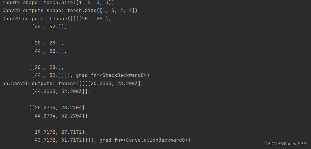
print('Conv2D outputs:', outputs)
# torch API运算结果
print('nn.Conv2D outputs:', outputs_torch)运行结果:
5.2.1.3 卷积算子的参数量和计算量
参数量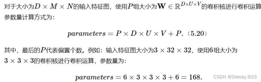
计算量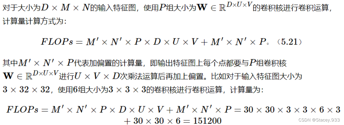
5.2.2汇聚层算子
汇聚层的作用是进行特征选择,降低特征数量,从而减少参数数量。由于汇聚之后特征图会变得更小,如果后面连接的是全连接层,可以有效地减小神经元的个数,节省存储空间并提高计算效率。
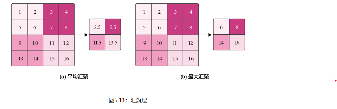
常用的汇聚方法有两种,分别是:平均汇聚和最大汇聚。
平均汇聚:将输入特征图划分为2×2大小的区域,对每个区域内的神经元活性值取平均值作为这个区域的表示;
最大汇聚:使用输入特征图的每个子区域内所有神经元的最大活性值作为这个区域的表示。
图5.11 给出了两种汇聚层的示例。
汇聚层输出的计算尺寸与卷积层一致,对于一个输入矩阵和一个运算区域大小为U×V的汇聚层,步长为S,对输入矩阵进行零填充,那么最终输出矩阵大小则为
由于过大的采样区域会急剧减少神经元的数量,也会造成过多的信息丢失。目前,在卷积神经网络中比较典型的汇聚层是将每个输入特征图划分为2×22×2大小的不重叠区域,然后使用最大汇聚的方式进行下采样。
由于汇聚是使用某一位置的相邻输出的总体统计特征代替网络在该位置的输出,所以其好处是当输入数据做出少量平移时,经过汇聚运算后的大多数输出还能保持不变。比如:当识别一张图像是否是人脸时,我们需要知道人脸左边有一只眼睛,右边也有一只眼睛,而不需要知道眼睛的精确位置,这时候通过汇聚某一片区域的像素点来得到总体统计特征会显得很有用。这也就体现了汇聚层的平移不变特性。
汇聚层的参数量和计算量
由于汇聚层中没有参数,所以参数量为0;最大汇聚中,没有乘加运算,所以计算量为0,而平均汇聚中,输出特征图上每个点都对应了一次求平均运算。
代码如下:
import torch
import torch.nn as nn

class Pool2D(nn.Module):
    def __init__(self, size=(2, 2), mode='max', stride=1):
        super(Pool2D, self).__init__()
        # 汇聚方式
        self.mode = mode
        self.h, self.w = size
        self.stride = stride

    def forward(self, x):
        output_w = (x.shape[2] - self.w) // self.stride + 1
        output_h = (x.shape[3] - self.h) // self.stride + 1
        output = torch.zeros([x.shape[0], x.shape[1], output_w, output_h])
        # 汇聚
        for i in range(output.shape[2]):
            for j in range(output.shape[3]):
                # 最大汇聚
                if self.mode == 'max':
                    output[:, :, i, j] = torch.max(
                        x[:, :, self.stride * i:self.stride * i + self.w, self.stride * j:self.stride * j + self.h])
                # 平均汇聚
                elif self.mode == 'avg':
                    output[:, :, i, j] = torch.mean(
                        x[:, :, self.stride * i:self.stride * i + self.w, self.stride * j:self.stride * j + self.h])

        return output


inputs = torch.tensor([[[[1., 2., 3., 4.], [5., 6., 7., 8.], [9., 10., 11., 12.], [13., 14., 15., 16.]]]])
pool2d = Pool2D(stride=2)
outputs = pool2d(inputs)
print("input: {}, \noutput: {}".format(inputs.shape, outputs.shape))

# 比较Maxpool2d与paddle API运算结果
maxpool2d_torch = nn.MaxPool2d(kernel_size=(2, 2), stride=2)
outputs_torch = maxpool2d_torch(inputs)
# 自定义算子运算结果
print('Maxpool2d outputs:', outputs)
# torch API运算结果
print('nn.Maxpool2d outputs:', outputs_torch)

# 比较Avgpool2D与torch API运算结果
avgpool2d_torch = nn.AvgPool2d(kernel_size=(2, 2), stride=2)
outputs_torch = avgpool2d_torch(inputs)
pool2d = Pool2D(mode='avg', stride=2)
outputs = pool2d(inputs)
# 自定义算子运算结果
print('Avgpool2d outputs:', outputs)
# paddle API运算结果
print('nn.Avgpool2d outputs:', outputs_torch)
运行结果:

选做题:使用pytorch实现Convolution Demo
1. 翻译以下内容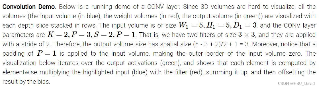
Convolution Demo.Below is a running demo of a CONV layer.Since 3D volumes are hard to visualize, all the volumes(the input volume(in bule),the weight volumes(in red),the output volumes(in green)) are visualized with each depth slice stacked in rows.The input volume is of size W1=5,H1=5,D1=3,and the CONV layer parameters are K=2,F=3,S=2,P=1.That is,have two filters of size 3 * 3,and they are applied with a stride of 2.Therefore,the output volume size has spatial size (5-3+2)/2+1=3. Moreover,notice that a padding of P=1 is applied to the input volume,making the outer border of the input volume zero.The visualizatin below iterates over the output activations (green),and shows that each element is computed by elementwise multiplying the highlighted input (blue) with the filter (red),summing it up,and then offsetting the result by the bias.
卷积演示。下面是一个 CONV 层的运行演示。由于 3D 体积难以可视化,因此所有体积(输入体积(蓝色)、重量体积(红色)、输出体积(绿色))都可视化,每个深度切片堆叠成行。输入音量大小W1=5,H1=5,D1=3W1=5,H1=5,D1=3,并且 CONV 图层参数为K=2,F=3,S=2,P=1K=2,F=3,S=2,P=1.也就是说,我们有两个大小的过滤器3×33×3,则以 2 的步幅应用它们。因此,输出卷大小具有空间大小 (5 - 3 + 2)/2 + 1 = 3。此外,请注意P=1P=1应用于输入音量,使输入音量的外部边界为零。下面的可视化效果循环访问输出激活(绿色),并显示每个元素的计算方法是将突出显示的输入(蓝色)与筛选器(红色)相乘,将其相加,然后通过偏差抵消结果。
2. 代码实现下图
使用卷积核Filter,代码如下:
import torch
import torch.nn as nn
class Conv2D(nn.Module):
def __init__(self, in_channels, out_channels, kernel_size, stride=1, padding=0, weight_attr=[], bias_attr=[]):
super(Conv2D, self).__init__()
self.weight = torch.nn.Parameter(weight_attr)
self.bias = torch.nn.Parameter(bias_attr)
self.stride = stride
self.padding = padding
# 输入通道数
self.in_channels = in_channels
# 输出通道数
self.out_channels = out_channels
# 基础卷积运算
def single_forward(self, X, weight):
# 零填充
new_X = torch.zeros([X.shape[0], X.shape[1] + 2 * self.padding, X.shape[2] + 2 * self.padding])
new_X[:, self.padding:X.shape[1] + self.padding, self.padding:X.shape[2] + self.padding] = X
u, v = weight.shape
output_w = (new_X.shape[1] - u) // self.stride + 1
output_h = (new_X.shape[2] - v) // self.stride + 1
output = torch.zeros([X.shape[0], output_w, output_h])
for i in range(0, output.shape[1]):
for j in range(0, output.shape[2]):
output[:, i, j] = torch.sum(
new_X[:, self.stride * i:self.stride * i + u, self.stride * j:self.stride * j + v] * weight,
axis=[1, 2])
return output
def forward(self, inputs):
"""
输入:
- inputs:输入矩阵,shape=[B, D, M, N]
- weights:P组二维卷积核,shape=[P, D, U, V]
- bias:P个偏置,shape=[P, 1]
"""
feature_maps = []
# 进行多次多输入通道卷积运算
p = 0
for w, b in zip(self.weight, self.bias): # P个(w,b),每次计算一个特征图Zp
multi_outs = []
# 循环计算每个输入特征图对应的卷积结果
for i in range(self.in_channels):
single = self.single_forward(inputs[:, i, :, :], w[i])
multi_outs.append(single)
# print("Conv2D in_channels:",self.in_channels,"i:",i,"single:",single.shape)
# 将所有卷积结果相加
feature_map = torch.sum(torch.stack(multi_outs), axis=0) + b # Zp
feature_maps.append(feature_map)
# print("Conv2D out_channels:",self.out_channels, "p:",p,"feature_map:",feature_map.shape)
p += 1
# 将所有Zp进行堆叠
out = torch.stack(feature_maps, 1)
return out
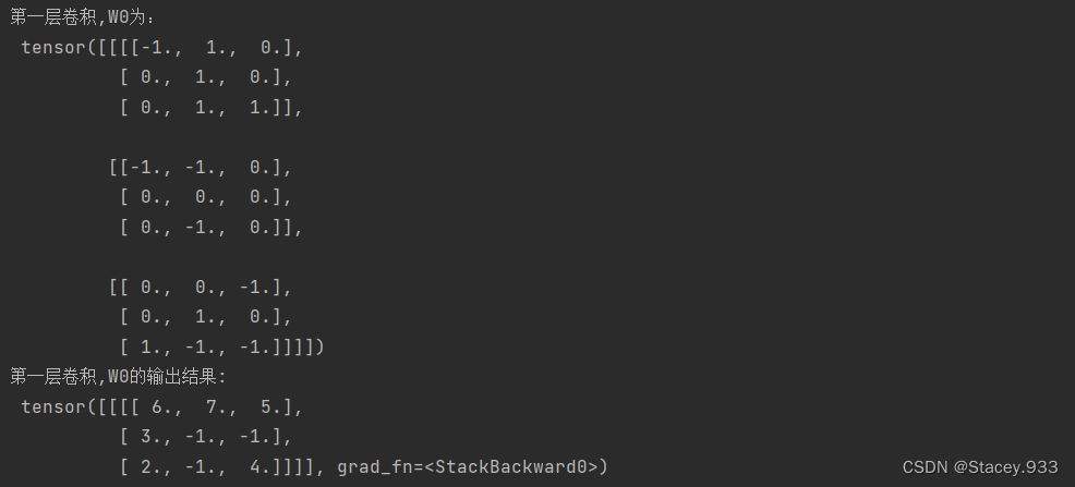
# 创建第一层卷积核
weight_attr1 = torch.tensor(
[[[-1, 1, 0], [0, 1, 0], [0, 1, 1]], [[-1, -1, 0], [0, 0, 0], [0, -1, 0]], [[0, 0, -1], [0, 1, 0], [1, -1, -1]]],
dtype=torch.float32)
weight_attr1 = weight_attr1.reshape([1, 3, 3, 3])
bias_attr1 = torch.tensor(torch.ones([3, 1]))
print("第一层卷积,W0为:\n", weight_attr1)
# 传入参数进行输出
Input_Volume = torch.tensor([[[0, 1, 1, 0, 2], [2, 2, 2, 2, 1], [1, 0, 0, 2, 0], [0, 1, 1, 0, 0], [1, 2, 0, 0, 2]]
, [[1, 0, 2, 2, 0], [0, 0, 0, 2, 0], [1, 2, 1, 2, 1], [1, 0, 0, 0, 0], [1, 2, 1, 1, 1]],
[[2, 1, 2, 0, 0], [1, 0, 0, 1, 0], [0, 2, 1, 0, 1], [0, 1, 2, 2, 2], [2, 1, 0, 0, 1]]])
Input_Volume = Input_Volume.reshape([1, 3, 5, 5])
conv2d_1 = Conv2D(in_channels=3, out_channels=3, kernel_size=3, stride=2, padding=1, weight_attr=weight_attr1,
bias_attr=bias_attr1)
output1 = conv2d_1(Input_Volume)
print("第一层卷积,W0的输出结果:\n", output1)
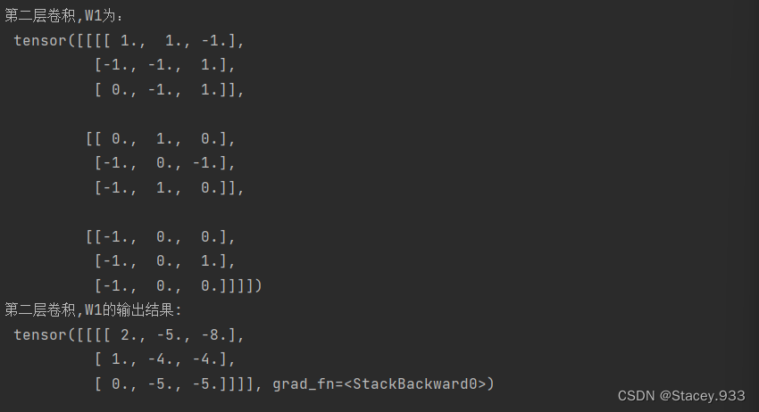
# 创建第二层卷积核
weight_attr2 = torch.tensor(
[[[1, 1, -1], [-1, -1, 1], [0, -1, 1]], [[0, 1, 0], [-1, 0, -1], [-1, 1, 0]], [[-1, 0, 0], [-1, 0, 1], [-1, 0, 0]]],
dtype=torch.float32)
weight_attr2 = weight_attr2.reshape([1, 3, 3, 3])
bias_attr2 = torch.tensor(torch.zeros([3, 1]))
print("第二层卷积,W1为:\n", weight_attr2)
Input_Volume = torch.tensor([[[0, 1, 1, 0, 2], [2, 2, 2, 2, 1], [1, 0, 0, 2, 0], [0, 1, 1, 0, 0], [1, 2, 0, 0, 2]]
, [[1, 0, 2, 2, 0], [0, 0, 0, 2, 0], [1, 2, 1, 2, 1], [1, 0, 0, 0, 0], [1, 2, 1, 1, 1]],
[[2, 1, 2, 0, 0], [1, 0, 0, 1, 0], [0, 2, 1, 0, 1], [0, 1, 2, 2, 2], [2, 1, 0, 0, 1]]])
Input_Volume = Input_Volume.reshape([1, 3, 5, 5])
conv2d_2 = Conv2D(in_channels=3, out_channels=2, kernel_size=3, stride=2, padding=1, weight_attr=weight_attr2,
bias_attr=bias_attr2)
output2 = conv2d_2(Input_Volume)
print("第二层卷积,W1的输出结果:\n", output2)运行结果:
总结:
本次实验主要是多通道卷积算子的实现和汇聚层算子的实现,了解了框架算子的使用方法,以及与自定义算子的区别,选做题整体的体会了一下利用不同卷积核提取不同特征的过程,对多通道卷积和汇聚有了更多理解。


 916
916


 被折叠的 条评论
为什么被折叠?
被折叠的 条评论
为什么被折叠?
 到【灌水乐园】发言


