看到Matrix67博客矩阵迭代分形,感觉不错

http://www.matrix67.com/blog/archives/500

矩阵、随机化与分形图形

    Stetson大学的一个非常可爱的MM（以后本Blog将简称她为Stetson MM）和我分享了一个很神奇的东西。她们正在做一个线性代数的课题研究，题目的大致意思是“用矩阵来构造分形图形”。Stetson MM叫我试着做下面这个实验：对于一个坐标点(x,y)，定义下面4个矩阵变换：
    
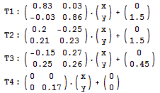
    然后，初始时令(x,y)等于(0,0)，按照 T1 – 85%, T2 – 6%, T3 – 8%, T4 – 1% 的概率，随机选择一个变换对该点进行操作，生成的点就是新的(x,y)；把它画在图上后，再重复刚才的操作，并一直这样做下去。

ClearAll["Global`*"];
list = {{0, 0}};
last = {{0}, {0}};
For[i = 0, i < 50000, i++, r = Random[];
 If[r < 0.85, 
  last = {{0.83, 0.03}, {-0.03, 0.86}}.last + {{0}, {1.5}}, 
  If[r < 0.91, 
   last = {{0.2, -0.25}, {0.21, 0.23}}.last + {{0}, {1.5}}, 
   If[r < 0.99, 
    last = {{-0.15, 0.27}, {0.25, 0.26}}.last + {{0}, {0.45}}, 
    last = {{0, 0}, {0, 0.17}}.last + {{0}, {0}}]]];
 list = Append[list, First[Transpose[last]]];]
h = ListPlot[list, PlotStyle -> {PointSize[0.002], Red}, 
   Axes -> False];
range = First /@ Differences /@ (PlotRange /. Options[h]);
Show[h, AspectRatio -> Last@range/First@range]

或者:

ClearAll["Global`*"];
list = {{0, 0}};
last = {{0}, {0}};
GetNextPoint[pt_] := Module[{r,
   t1 = {{0.83, 0.03}, {-0.03, 0.86}}, p1 = {0, 1.5},
   t2 = {{0.2, -0.25}, {0.21, 0.23}}, p2 = {0, 1.5},
   t3 = {{-0.15, 0.27}, {0.25, 0.26}}, p3 = {0, 0.45},
   t4 = {{0, 0}, {0, 0.17}}, p4 = {0, 0}},
  r = Random[];
  If[r <= 0.85, t1.pt + p1, 
   If[r <= 0.91, t2.pt + p2, If[r <= 0.99, t3.pt + p3, t4.pt + p4]]]]
For[i = 0, i < 50000, i++, last = GetNextPoint[last];
 list = Append[list, First[Transpose[last]]];]
h = ListPlot[list, PlotStyle -> {PointSize[0.005], Red}, 
   Axes -> False];
range = First /@ Differences /@ (PlotRange /. Options[h]);
Show[h, AspectRatio -> Last@range/First@range]

ClearAll["Global`*"];
t0 = AbsoluteTime[];
list = {{0, 0}};
last = {{0}, {0}};
GetNextPoint[pt_] := 
 Module[{r, 
   t1 = Transpose[
     Reverse[Transpose[Reverse[{{0.83, 0.03}, {-0.03, 0.86}}]]]], 
   p1 = Reverse[{0, 1.5}], 
   t2 = Transpose[
     Reverse[Transpose[Reverse[{{0.2, -0.25}, {0.21, 0.23}}]]]], 
   p2 = Reverse[{0, 1.5}], 
   t3 = Transpose[
     Reverse[Transpose[Reverse[{{-0.15, 0.27}, {0.25, 0.26}}]]]], 
   p3 = Reverse[{0, 0.45}], 
   t4 = Transpose[Reverse[Transpose[Reverse[{{0, 0}, {0, 0.17}}]]]], 
   p4 = Reverse[{0, 0}]}, r = Random[];
  If[r <= 0.85, t1.pt + p1, 
   If[r <= 0.91, t2.pt + p2, If[r <= 0.99, t3.pt + p3, t4.pt + p4]]]]
For[i = 0, i < 100000, i++, last = GetNextPoint[last];
 list = Append[list, First[Transpose[last]]];]
h = ListPlot[list, PlotStyle -> {PointSize[0.002], Green}, 
   Axes -> False, Background -> Black];
range = First /@ Differences /@ (PlotRange /. Options[h]);
Show[h, AspectRatio -> Last@range/First@range]
Print[AbsoluteTime[] - t0]

用下面的代码可以提速数十倍:

Clear["`*"];
t0 = AbsoluteTime[];
ifs[prob_, A_, init_, maxIter_] := 
  FoldList[#2.{#[[1]], #[[2]], 1} &, init, 
   RandomChoice[prob -> A, maxIter]];

init = {0., 0.};
prob = N@{85, 6, 8, 1};
A = N@{{{0.83, 0.03, 0}, {-0.03, 0.86, 1.5}}, {{0.2, -0.25, 0}, {0.21,
       0.23, 1.5}}, {{-0.15, 0.27, 0}, {0.25, 0.26, 0.45}}, {{0, 0, 
      0}, {0, 0.17, 0}}};
iter = 10^5;
pts = ifs[prob, A, init, iter];
Graphics[{PointSize[0.002], Green, Point[pts]}, Background -> Black]
(*h=ListPlot[pts,PlotStyle\[Rule]Green,Background\[Rule]Black];
range=First/@Differences/@(PlotRange/.Options[h]);Show[h,AspectRatio\
\[Rule]Last@range/First@range,Axes->False]*)
Print[AbsoluteTime[] - t0]

这类经典问题,维基上总是有答案的:

http://en.wikipedia.org/wiki/Barnsley_fern

The Barnsley Fern is a fractal named after the British mathematician Michael Barnsley who first described it in his bookFractals Everywhere.^[1] He made it to resemble the Black Spleenwort, Asplenium adiantum-nigrum.

History[edit]

The fern is one of the basic examples of self-similar sets, i.e. it is a mathematically generated pattern that can be reproducible at any magnification or reduction. Like the Sierpinski triangle, the Barnsley fern shows how graphically beautiful structures can be built from repetitive uses of mathematical formulas with computers. Barnsley's book about fractals is based on the course which he taught for undergraduate and graduate students in the School of Mathematics, Georgia Institute of Technology, called Fractal Geometry. After publishing the book, a second course was developed, called Fractal Measure Theory.^[1] Barnsley's work has been a source of inspiration to graphic artists attempting to imitate nature with mathematical models.

The fern code developed by Barnsley is an example of an iterated function system (IFS) to create a fractal. He has used fractals to model a diverse range of phenomena in science and technology, but most specifically plant structures.

"IFSs provide models for certain plants, leaves, and ferns, by virtue of the self-similarity which often occurs in branching structures in nature. But nature also exhibits randomness and variation from one level to the next; no two ferns are exactly alike, and the branching fronds become leaves at a smaller scale. V-variable fractals allow for such randomness and variability across scales, while at the same time admitting a continuous dependence on parameters which facilitates geometrical modelling. These factors allow us to make the hybrid biological models...

...we speculate that when a V -variable geometrical fractal model is found that has a good match to the geometry of a given plant, then there is a specific relationship between these code trees and the information stored in the genes of the plant.

—Michael Barnsley et al.^[2]

Construction[edit]

Real lady ferns.

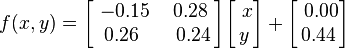
Barnsley's fern uses four affine transformations. The formula for one transformation is the following:

Barnsley shows the IFS code for his Black Spleenwort fern fractal as a matrix of values shown in a table.^[1] In the table, the columns "a" through "f" are the coefficients of the equation, and "p" represents the probability factor.

w	a	b	c	d	e	f	p
ƒ1	0	0	0	0.16	0	0	0.01
ƒ2	0.85	0.04	−0.04	0.85	0	1.6	0.85
ƒ3	0.2	−0.26	0.23	0.22	0	1.6	0.07
ƒ4	−0.15	0.28	0.26	0.24	0	0.44	0.07

These correspond to the following transformations:

Computer generation[edit]

Fractal fern in four states of construction. Highlighted triangles show how the half of one  leaflet is transformed to half of one whole leaf or  frond.

Though Barnsley's fern could in theory be plotted by hand with a pen and graph paper, the number of iterations necessary runs into the tens of thousands, which makes use of a computer practically mandatory. Many different computer models of Barnsley's fern are popular with contemporary mathematicians. As long as the math is programmed correctly using Barnsley's matrix of constants, the same fern shape will be produced.

The first point drawn is at the origin (x₀ = 0, y₀ = 0) and then the new points are iteratively computed by randomly applying one of the following four coordinate transformations:^[3][4]

ƒ₁

x _{n + 1} = 0

y _{n + 1} = 0.16  y _n.

This coordinate transformation is chosen 1% of the time and just maps any point to a point in the first line segment at the base of the stem. This part of the figure is the first to be completed in during the course of iterations.

ƒ₂

x _{n + 1} = 0.85  x _n + 0.04  y _n

y _{n + 1} = −0.04  x _n + 0.85  y _n + 1.6.

This coordinate transformation is chosen 85% of the time and maps any point inside the leaflet represented by the red triangle to a point inside the opposite, smaller leaflet represented by the blue triangle in the figure.

ƒ₃

x _{n + 1} = 0.2  x _n − 0.26  y _n

y _{n + 1} = 0.23  x _n + 0.22  y _n + 1.6.

This coordinate transformation is chosen 7% of the time and maps any point inside the leaflet (or pinna) represented by the blue triangle to a point inside the alternating corresponding triangle across the stem (it flips it).

ƒ₄

x _{n + 1} = −0.15  x _n + 0.28  y _n

y _{n + 1} = 0.26  x _n + 0.24  y _n + 0.44.

This coordinate transformation is chosen 7% of the time and maps any point inside the leaflet (or pinna) represented by the blue triangle to a point inside the alternating corresponding triangle across the stem (without flipping it).

The first coordinate transformation draws the stem. The second generates successive copies of the stem and bottom fronds to make the complete fern. The third draws the bottom frond on the left. The fourth draws the bottom frond on the right. The recursive nature of the IFS guarantees that the whole is a larger replica of each frond. Note that the complete fern is within the range −2.1820 < x < 2.6558 and 0 ≤ y < 9.9983.

Mutant varieties[edit]

Barnsley fern mutated into a Thelypteridaceae fern.

Barnsley fern mutated into a leptosporangiate fern.

By playing with the coefficients, it is possible to create mutant fern varieties. In his paper on V-variable fractals, Barnsley calls this trait a superfractal.^[2]

One experimenter has come up with a table of coefficients to produce another remarkably naturally looking fern however, resembling the Cyclosorus or Thelypteridaceae fern. These are:^[5][6]

w	a	b	c	d	e	f	p
ƒ1	0	0	0	0.25	0	−0.4	0.02
ƒ2	0.95	0.005	−0.005	0.93	−0.002	0.5	0.84
ƒ3	0.035	−0.2	0.16	0.04	−0.09	0.02	0.07
ƒ4	−0.04	0.2	0.16	0.04	0.083	0.12	0.07

References[edit]

1. ^ Jump up to:^a b c Fractals Everywhere, Boston, MA: Academic Press, 1993, ISBN 0-12-079062-9
2. ^ Jump up to:^a b Michael Barnsley, et al.,"V-variable fractals and superfractals" PDF (2.22 MB)
3. Jump up^ Barnsley, Michael (2000). Fractals everywhere. Morgan Kaufmann. p. 86. ISBN 0-12-079069-6. Retrieved 2010-01-07.
4. Jump up^ Weisstein, Eric. "Barnsley's Fern". Retrieved 2010-01-07.
5. Jump up^ Other fern varieties with supplied coefficients, retrieved 2010-1-7
6. Jump up^ A Barnsley fern generator

漂亮的网页生成该分形的html5工具:

http://www.chradams.co.uk/fern/maker.html