K邻近算法

最新推荐文章于 2023-10-09 21:55:53 发布

_tommy

最新推荐文章于 2023-10-09 21:55:53 发布

阅读量668

点赞数

分类专栏：机器学习文章标签：机器学习

本文链接：https://blog.csdn.net/stromcruise/article/details/78251235

版权

机器学习专栏收录该内容

3 篇文章 0 订阅

订阅专栏

机器学习实战

本章内容：

K-近邻分类算法
从文本文件中解析和导入数据
使用 Matplotlib创建扩散图
归一化数值

k-近邻算法概述

原理：k-近邻算法采用测量不同特征值之间的距离方法进行分类

优点：精度高、对异常值不敏感、无数据输入假定
缺点：计算复杂度高，空间复杂度高
适用数据范围：数值型和标称型

工作原理：存在一个样本数据集合，也称作训练要样本集合，并且样本集合中每个数据都存在标签，即我们知道样本集中每一数据与所属分类的对应关系。输入没有标签的新数据后，将新数据的每个特征与样本集中数据对应的特征进行比较，然后算法提取样本集中特征最相似（即最近邻）的分类标签。一般来说，我们只选择样本集合中前k个最相似的数据，这就是k-近邻算法中k的出处，通常k是不超多20的整数。最后选择k个数据中出现次数最多的分类标签作为新数据的分类。

Python实现近邻算法

k-近邻算法的一般流程

收集数据：可以使用任何方法
准备数据：距离计算所需要的数值，最好是结构化的数据格式
分析数据：可以使用任何方法
训练算法：不适用k近邻算法
测试算法：计算错误率
使用算法：首先需要输入样本数据和结构化的输出结果，然后运行k-近邻算法判定输入数据分别属于哪个分类，最后应用对计算出的分类执行后续的处理。

准备：使用python 导入数据

以下代码过程均在pycharm 中运行
Python3.6.1

创建 KNN.py 文件

from numpy import *    # 科学计算包
import operator         # 运算符模块
def createDataSet():
    group = array([[1.0,1.1],[1.0,1.0],[0,0],[0,0.1]])
    labels = ['A','A','B','B']
    return group, labels

group,labels = createDateDataSet()
group为数据特征值，labels为标签分类。

从文本文件中解析数据

本节使用程序清单2-1的函数运行KNN算法，为每组数据分类。这里首先给出k-近邻算法的伪代码和实际Python代码，然后详细解释每行代码的含义。该函数的功能是使用k-近邻算法将每组数据划分到某个类中，其伪代码如下：

对未知类别属性的数据集中的每个点依次执行以下操作：

计算已知类别数据集中点与当前点之间的距离；
按照距离递增次序排序；
选取与当前点距离最小的k个点；
确定前k个点所在类别的出现频率；
返回前k个点中出现频率最高的类别作为当前点的预测分类

程序清单2-1 k-近邻算法

def classify0(inX, dataSet, labels, k):
    dataSetSize = dataSet.shape[0] 
    diffMat = tile(inX, (dataSetSize,1)) - dataSet  
    sqDiffMat = diffMat**2
    sqDistances = sqDiffMat.sum(axis=1)
    distances = sqDistances**0.5
    sortedDistIndicies = distances.argsort()     
    classCount={}          
    for i in range(k):
        voteIlabel = labels[sortedDistIndicies[i]]
        classCount[voteIlabel] = classCount.get(voteIlabel,0) + 1
    sortedClassCount = sorted(classCount.items(), key=operator.itemgetter(1), reverse=True)
    return sortedClassCount[0][0]

classify0() 函数具有四个参数：用于分类的输入向量是inX,输入的训练样本集为dataSet, 标签向量为labels，最后参数k表示用于选择最邻近的数量，其中标签向量的元素数目和矩阵dataSet的行数相同。使用的是欧式距离公式。

group,labels = createDataSet()
l = classify0([0,0],group,labels,3)
print(l)

运行上述代码，很明显[0,0] 被分到B类。

实际案列

一：案例应用场景如下：

我的朋友海伦一直使用在线约会网站寻找合适自己的约会对象。尽管约会网站会推荐不同的人选，但她并不是喜欢每一个人。经过一番总结，她发现曾交往过三种类型的人：
（1）不喜欢的人；
（2）魅力一般的人；
（3）极具魅力的人；
尽管发现了上述规律，但海伦依然无法将约会网站推荐的匹配对象归入恰当的分类，她觉得可以在周一到周五约会那些魅力一般的人，而周末则更喜欢与那些极具魅力的人为伴。海伦希望我们的分类软件可以更好地帮助她将匹配对象划分到确切的分类中。此外，海伦还收集了一些约会网站未曾记录的数据信息，她认为这些数据更助于匹配对象的归类。

二：在约会网站上使用KNN邻近算法

（1）收集数据：提供文本文件；
（2）准备数据：使用Python解析文本文件；
（3）分析数据：使用Matplotlib画二维扩散图；
（4）训练算法：此步骤不适用于K-近邻算法；
（5）测试算法：使用海伦提供的部分数据作为测试样本，
测试样本和非测试样本的区别在于：测试样本是已经完成分类的数据，如果预测分类与实际类别不同，则标记为一个错误。
（6）使用算法：产生简单的命令行程序，然后海伦可以输入一些特征数据以判断对方是否为自己喜欢的类型。

海伦收集约会数据已经有了一段时间，她把这些数据存放在文本文件datingTestSet.txt中，每个样本数据占据一行，总共有1000行。海伦的样本主要包括以下3种特征：
1.每年获得的飞行常客里程数；
2.玩视频游戏所耗时间百分比；
3.每周消费的冰淇淋公升数；
在将上述特征数据输入到分类器之前，必须将待处理数据的格式改变为分类器可以接受的格式。在kNN.py中创建名为file2matrix的函数，以此来处理输入格式问题。该函数的输入为文本文件名字符串，输出为训练样本矩阵和类标签向量。

程序清单2-2 将文本记录到转化Numpy的解析程序

def file2matrix(filename):
    fr = open(filename)
    numberOfLines = len(fr.readlines())         #get the number of lines in the file
    returnMat = zeros((numberOfLines,3))        #prepare matrix to return
    classLabelVector = []                       #prepare labels return
    fr = open(filename)
    index = 0
    for line in fr.readlines():
        line = line.strip()
        listFromLine = line.split('\t')
        returnMat[index,:] = listFromLine[0:3]
        classLabelVector.append(int(listFromLine[-1]))
        index += 1
    return returnMat,classLabelVector

filename = r’./datingTestSet2.txt’
datingDataMat,datingLabels = file2matrix(filename)
print(datingDataMat)

[[  4.09200000e+04   8.32697600e+00   9.53952000e-01]
 [  1.44880000e+04   7.15346900e+00   1.67390400e+00]
 [  2.60520000e+04   1.44187100e+00   8.05124000e-01]
 ..., 
 [  2.65750000e+04   1.06501020e+01   8.66627000e-01]
 [  4.81110000e+04   9.13452800e+00   7.28045000e-01]
 [  4.37570000e+04   7.88260100e+00   1.33244600e+00]]

三：分析数据：使用Matplotlib创建散点图

import matplotlib  
import matplotlib.pyplot as plt 
def showPic():
    zhfont = matplotlib.font_manager.FontProperties(fname='D:\\fonts\\STXINGKA.TTF')  # 字体
    fig = plt.figure()
    ax = fig.add_subplot(111)
    ax.scatter(datingDataMat[:,1],datingDataMat[:,2],
           15.0*array(datingLabels),15.0*array(datingLabels))
    plt.xlabel(u'玩游戏所耗时间百分比', fontproperties=zhfont)
    plt.ylabel(u'每周消费的冰淇淋公升数', fontproperties=zhfont)
    plt.show()

showPic()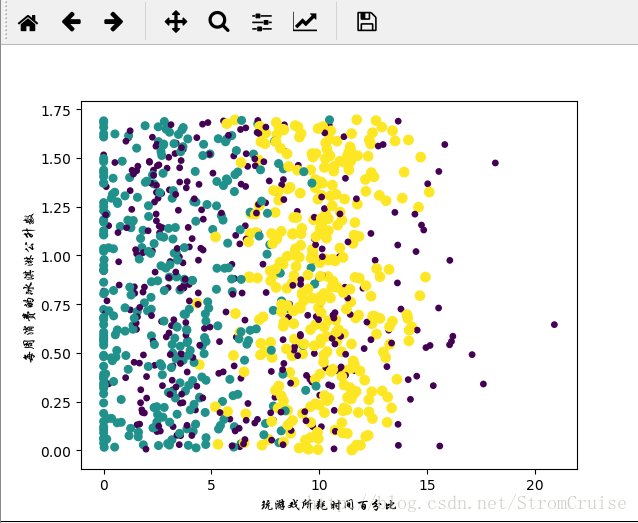

这里写图片描述

上图是带有样本分类标签的约会数据散点图，虽然能够比较容易地区分数据点从属类别，但依然很难根据这张图得出结论信息。

上图使用了datingDataMat矩阵属性列2和列3展示数据，虽然也可以区别，但下图采用列1和列2的属性值却可以得到更好的效果：

def showPic2():
    zhfont = matplotlib.font_manager.FontProperties(fname='D:\\fonts\\STXINGKA.TTF')
    plt.figure(figsize=(8, 5), dpi=80)
    ax = plt.subplot(111)
    # 将三类数据分别取出来
    # x轴代表飞行的里程数
    # y轴代表玩视频游戏的百分比
    type1_x = []
    type1_y = []
    type2_x = []
    type2_y = []
    type3_x = []
    type3_y = []
    print( 'range(len(labels)):',end='  ')
    print(range(len(datingLabels)))
    for i in range(len(datingLabels)):
        if datingLabels[i] == 1:  # 不喜欢
            type1_x.append(datingDataMat[i][0])
            type1_y.append(datingDataMat[i][1])

        if datingLabels[i] == 2:  # 魅力一般
            type2_x.append(datingDataMat[i][0])
            type2_y.append(datingDataMat[i][1])

        if datingLabels[i] == 3:  # 极具魅力
            print("===",i, '：', datingLabels[i], ':', type(datingLabels[i]))
            type3_x.append(datingDataMat[i][0])
            type3_y.append(datingDataMat[i][1])

    type1 = ax.scatter(type1_x, type1_y, s=20, c='red')
    type2 = ax.scatter(type2_x, type2_y, s=40, c='green')
    type3 = ax.scatter(type3_x, type3_y, s=50, c='blue')
    # plt.scatter(matrix[:, 0], matrix[:, 1], s=20 * numpy.array(labels),
    #             c=50 * numpy.array(labels), marker='o',
    #             label='test')
    plt.xlabel(u'每年获取的飞行里程数', fontproperties=zhfont)
    plt.ylabel(u'玩视频游戏所消耗的事件百分比', fontproperties=zhfont)
    ax.legend((type1, type2, type3), (u'不喜欢', u'魅力一般', u'极具魅力'), loc=2, prop=zhfont)
    plt.show()

showPic2()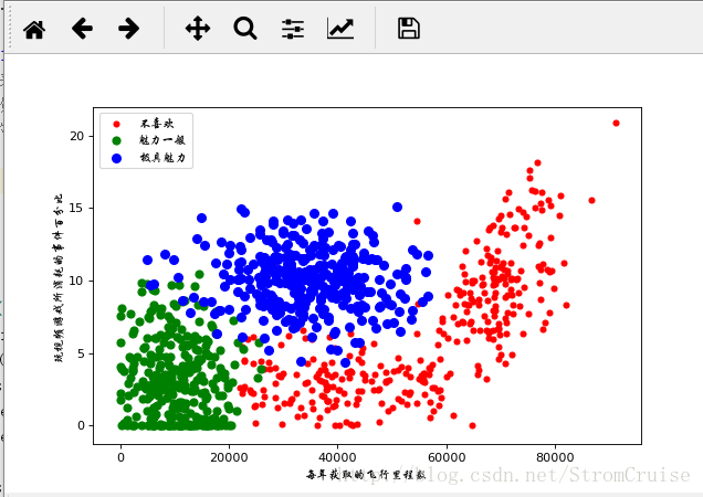

这里写图片描述

图中清晰的标识了三个不同的样本分类区域，具有不同爱好的人其类别区域也不同，可以看出用图中展示的“每年获取飞行常客里程数”和“玩视频游戏所耗时间百分比”两个特征更容易区分数据点从属的类别。

四：准备数据：归一化数值
我们很容易想到计算样本之间的距离，当某个维度过大时，会对计算结果造成很大影响，所以要对数值进行归一化处理。
归一到[0,1]

def autoNorm(dataSet):
    minVals = dataSet.min(0)
    maxVals = dataSet.max(0)
    ranges = maxVals - minVals
    normDataSet = zeros(shape(dataSet))
    m = dataSet.shape[0]
    normDataSet = dataSet - tile(minVals, (m,1))
    normDataSet = normDataSet/tile(ranges, (m,1))   #element wise divide
    return normDataSet, ranges, minVals

normDataSet, ranges, minVals =  autoNorm(dataSet=datingDataMat)
print(normDataSet)

运行代码得到如下结果：

[[ 0.44832535  0.39805139  0.56233353]
 [ 0.15873259  0.34195467  0.98724416]
 [ 0.28542943  0.06892523  0.47449629]
 ..., 
 [ 0.29115949  0.50910294  0.51079493]
 [ 0.52711097  0.43665451  0.4290048 ]
 [ 0.47940793  0.3768091   0.78571804]]

五：测试算法：作为完整程序验证分类器
机器学习算法中一个很重要的工作就是评估算法的正确率，通常我们会将已有数据的90%作为训练样本来训练分类器，而使用其余10%的数据去测试分类器，检测分类器的正确率。这里是用的50%
1.分类器对约会网站的测试代码：

def datingClassTest():
    hoRatio = 0.50      #hold out 10%
    datingDataMat,datingLabels = file2matrix('datingTestSet2.txt')       #load data setfrom file
    normMat, ranges, minVals = autoNorm(datingDataMat)
    m = normMat.shape[0]
    numTestVecs = int(m*hoRatio)
    errorCount = 0.0
    for i in range(numTestVecs):
        classifierResult =  classify0(normMat[i,:],normMat[numTestVecs:m,:]
                           ,datingLabels[numTestVecs:m],3)
        print("the classifier came back with: %d, the real answer is: %d" %
                            (classifierResult, datingLabels[i]))
        if (classifierResult != datingLabels[i]): errorCount += 1.0
    print("the total error rate is: %f" % (errorCount/float(numTestVecs)))
    print(errorCount)

datingClassTest()

the classifier came back with: 3, the real answer is: 3
the classifier came back with: 2, the real answer is: 2
the classifier came back with: 1, the real answer is: 1
the classifier came back with: 1, the real answer is: 1
the classifier came back with: 1, the real answer is: 1
the classifier came back with: 1, the real answer is: 1
the classifier came back with: 3, the real answer is: 3
the classifier came back with: 3, the real answer is: 3
...
the classifier came back with: 1, the real answer is: 1
the classifier came back with: 2, the real answer is: 1
the classifier came back with: 2, the real answer is: 2
the classifier came back with: 1, the real answer is: 1
the classifier came back with: 1, the real answer is: 1
the classifier came back with: 2, the real answer is: 2
the total error rate is: 0.066000
33.0

可见分类的正确率还是很高的，达到99%以上，之分类错了33个，总测试样本（500）

六：使用算法：构建完整可用系统。

输入某人信息，预测出海伦对对方喜欢程度：

def classifyPerson():  
    resultList=['not at all','in small doses','in large doses']  
    percentTats=float(input("percentage of time spent playing video games?"))  
    ffMiles=float(input("frequent flier miles earned per year?"))  
    iceCream=float(input("liters of ice cream consumed per year?"))  
    datingDataMat,datingLabels=file2matrix('datingTestSet2.txt')  
    normMat,ranges,minVals=autoNorm(datingDataMat)  
    inArr=array([ffMiles,percentTats,iceCream])  
    classifierResult=classify0((inArr-minVals)/ranges,normMat,datingLabels,3)  
    print "You will probably like this person:",resultList[classifierResult-1] 

classifyPerson()

运行输入如下：

percentage of time spent playing video games?10
frequent flier miles earned per year?40000
liters of ice cream consumed per year?1
You will probably like this person: in large doses

Process finished with exit code 0

上述代码中涉及到的有些函数：Python中排序常用到的sort 、sorted和argsort函数
http://blog.csdn.net/u013731339/article/details/41449177

Python-Numpy的tile函数用法
http://www.cnblogs.com/zibu1234/p/4210521.html

_tommy

关注

0
点赞
踩
1

收藏

觉得还不错? 一键收藏
0
评论
K邻近算法

机器学习实战本章内容：K-近邻分类算法从文本文件中解析和导入数据使用 Matplotlib创建扩散图归一化数值k-近邻算法概述原理：k-近邻算法采用测量不同特征值之间的距离方法进行分类优点：精度高、对异常值不敏感、无数据输入假定缺点：计算复杂度高，空间复杂度高适用数据范围：数值型和标称型工作原理：存在一个样本数据集合，也称作训练要样本集合
复制链接

扫一扫