numpy总结与思维导图

最新推荐文章于 2023-09-02 23:11:14 发布

submarineas

最新推荐文章于 2023-09-02 23:11:14 发布

阅读量5.2k

点赞数 18

分类专栏： python 文章标签： numpy

本文链接：https://blog.csdn.net/submarineas/article/details/85041240

版权

python 专栏收录该内容

64 篇文章 19 订阅

订阅专栏

引言
numpy语法总结
- numpy基础思维导图
- 部分解释
高阶部分
总结

引言

本文基于《基于python进行数据分析》与实验楼中的numpy实验，针对其中的一些基础知识与问题，结合自己的一些经验，进行了汇总，在这里写下一个总结。

什么是numpy？

NumPy是高性能科学计算和数据分析的基础包。部分功能如下：

ndarray, 具有矢量算术运算和复杂广播能力的快速且节省空间的多维数组。
用于对整组数据进行快速运算的标准数学函数（无需编写循环）。
用于读写磁盘数据的工具以及用于操作内存映射文件的工具。
线性代数、随机数生成以及傅里叶变换功能。
用于集成C、C++、Fortran等语言编写的代码的工具。

numpy优势

我们可以看下面的图：
在这里插入图片描述
这张图来自百度百科，我们可以发现的是array类型数据存储方式是连续的，并且直接指代，而列表的线反而显得杂乱无章，还需要通过寻址来存储，这就导致了numpy在计算的时候虽然类型单一，但没有太多循环的限制，还有可执行向量化操作与解决了GIL全局解释器锁，都给它的速度带来了质的飞越。

另外我记得在看哪本书中提到过，python列表实际上是数组，具体来说，它们是具有指数过度分配的动态数组，可分离的顺序表。python创始人龟叔在编写cpython解释器的过分分配非常保守，只给了1.125倍的速率，这在大部分语言里，是比较低的。
(书不记得哪本了，翻找了很多的资料，在quora上找到一个讨论帖，可以一看 How-are-Python-lists-implemented-internally)

关于numpy的缺点，可以看这篇博文：
numpy 矩阵运算的陷阱

ndarray的类型

类型	类型代码	说明
int8、uint8	i1、u1	有符号和无符号8位整型（1字节）
int16、uint16	i2、u2	有符号和无符号16位整型（2字节）
int32、uint32	i4、u4	有符号和无符号32位整型（4字节）
int64、uint64	i8、u8	有符号和无符号64位整型（8字节）
float16	f2	半精度浮点数
float32	f4、f	单精度浮点数
float64	f8、d	双精度浮点数
float128	f16、g	扩展精度浮点数
complex64	c8	分别用两个32位表示的复数
complex128	c16	分别用两个64位表示的复数
complex256	c32	分别用两个128位表示的复数
bool	?	布尔型
object	O	python对象
string	Sn	固定长度字符串，每个字符1字节，如S10
unicode	Un	固定长度Unicode，字节数由系统决定，如U10

是不是有点晕？我做完表也有点。其实不需要考虑这么多，只要知道它支持很多种格式，有整形、浮点型、复数这三个就差不多了。其它的用得少。

numpy语法总结

numpy基础思维导图

在这里插入图片描述
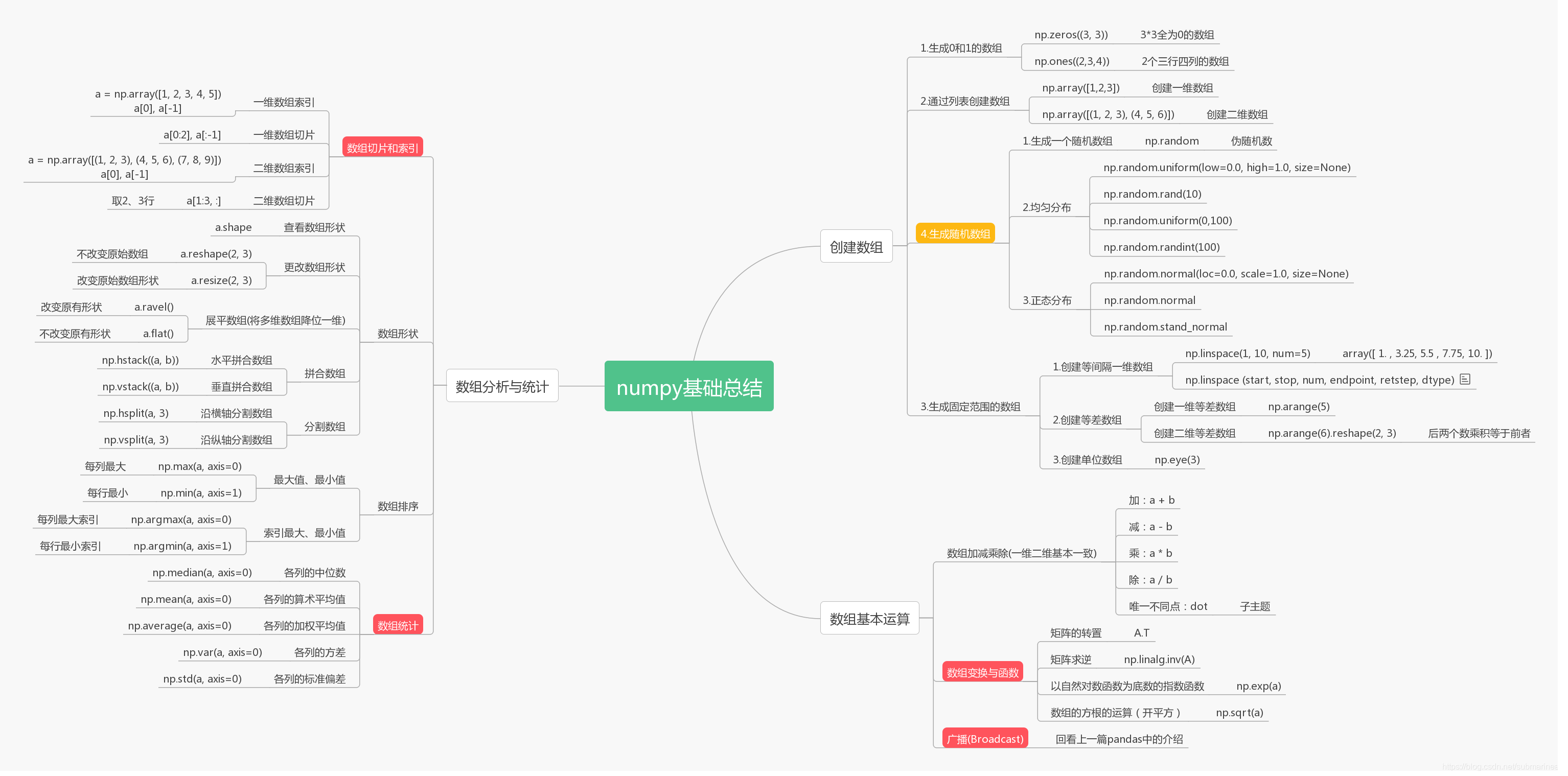
图中大部分是我对一些基础性的东西进行的总结，大部分是印象流，大概过一遍就差不太多了。下面我就挑一些出来分析：

部分解释

1. 正态分布：
什么是正态分布？大体来讲就是如下公式：
$\frac{1}{\sqrt{2\pi }\sigma }e^{-\frac{(x-\mu )^{2}}{2\sigma ^{2}}}$

具体的我们可以看如下链接：
The Standard Normal Distribution

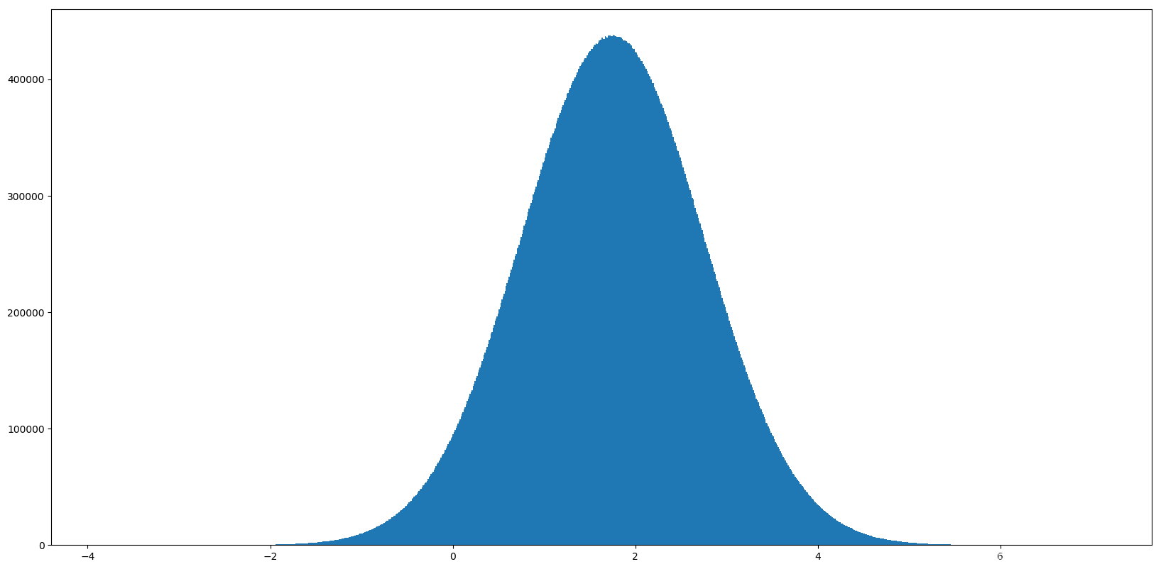
然后当我们懂了什么是正态分布，下面就可以自己来模拟一个图了：

import matplotlib.pyplot as plt
import numpy as np

# 生成均匀分布的随机数
x2 = np.random.normal(1.75, 1, 100000000)
# 创建画布
plt.figure(figsize=(20, 10), dpi=100)
# 绘制直方图
plt.hist(x2, 1000)
# 显示图像
plt.show()

图形如下：
在这里插入图片描述

2. 垂直拼合数组与水平合并

# 生成示例数组
a = np.random.randint(10, size=(3, 3))
b = np.random.randint(10, size=(3, 3))
a, b
"""
(array([[7, 0, 8],
        [9, 4, 7],
        [3, 3, 8]]), array([[8, 5, 6],
        [6, 0, 1],
        [6, 9, 4]]))
"""

np.vstack((a, b))	# 垂直合并
"""
array([[7, 0, 8],
       [9, 4, 7],
       [3, 3, 8],
       [8, 5, 6],
       [6, 0, 1],
       [6, 9, 4]])
"""

np.hstack((a, b))	# 水平合并
"""
array([[7, 0, 8, 8, 5, 6],
       [9, 4, 7, 6, 0, 1],
       [3, 3, 8, 6, 9, 4]])
"""

3. 返回每列最大每行最小

print(a)
np.min(a, axis=1)	# 返回每行最小值
"""
[[7 0 8]
 [9 4 7]
 [3 3 8]]
Out[30]:
array([0, 4, 3])
"""

np.max(a, axis=0)	# 返回每列最大值
"""
array([9, 4, 8])
"""
np.max(a,axis=1)	# 返回每行最小值

4. 矩阵求逆：

A = np.array([[1, 2],
              [3, 4]])
np.linalg.inv(A)
"""
array([[-2. ,  1. ],
       [ 1.5, -0.5]])
"""

5. 均匀分布：
均匀分布就不用说了，可以见下图：

# 生成均匀分布的随机数
x1 = np.random.uniform(-1, 1, 100000000)
# 1）创建画布
plt.figure(figsize=(10, 10), dpi=100)
# 2）绘制直方图
plt.hist(x1, 5000)
# 3）显示图像
plt.show()

在这里插入图片描述

高阶部分

熟悉使用技巧

1. 创建一个 0-10 的一维数组，并将 (1, 9] 之间的数全部反转成负数：

Z = np.arange(11)
Z[(1 < Z) & (Z <= 9)] *= -1
Z
"""
array([ 0,  1, -2, -3, -4, -5, -6, -7, -8, -9, 10])
"""

2. 找出两个一维数组中相同的元素：

Z1 = np.random.randint(0,10,10)
Z2 = np.random.randint(0,10,10)
print("Z1:", Z1)
print("Z2:", Z2)
np.intersect1d(Z1,Z2)	# 返回Z1和Z2中的交集
"""
Z1: [6 3 7 9 2 0 1 1 3 3]
Z2: [0 4 8 1 5 8 5 0 6 5]
array([0, 1, 6])
"""

3. 创建一个长度为10的随机一维数组，并将其按升序排序：

Z = np.random.random(10)
Z.sort()
Z
"""
array([0.06298303, 0.12848206, 0.26675583, 0.36847405, 0.6276631 ,
       0.73499294, 0.73732823, 0.83748245, 0.85359826, 0.91563148])
"""

4. 使用 NumPy 打印昨天、今天、明天的日期：

yesterday = np.datetime64('today', 'D') - np.timedelta64(1, 'D')
today     = np.datetime64('today', 'D')
tomorrow  = np.datetime64('today', 'D') + np.timedelta64(1, 'D')
print("yesterday: ", yesterday)
print("today: ", today)
print("tomorrow: ", tomorrow)

"""
yesterday:  2018-12-21
today:  2018-12-22
tomorrow:  2018-12-23
"""

5. 使用五种不同的方法去提取一个随机数组的整数部分：

Z = np.random.uniform(0,10,10)		# 均匀分布的随机数
print("原始值: ", Z)
print ("方法 1: ", Z - Z%1)			# 减去余数
print ("方法 2: ", np.floor(Z))		# 逐元素的返回输入的下限
print ("方法 3: ", np.ceil(Z)-1)		# 计算大于等于改值的最小整数
print ("方法 4: ", Z.astype(int))	# Z.astype
print ("方法 5: ", np.trunc(Z))		# 按元素方式返回输入的截断值
"""
原始值:  [1.53413298 2.71912419 9.74111772 3.67325886 7.62381231 3.74703012
 8.33338283 0.4819538  5.48684884 1.8034668 ]
方法 1:  [1. 2. 9. 3. 7. 3. 8. 0. 5. 1.]
方法 2:  [1. 2. 9. 3. 7. 3. 8. 0. 5. 1.]
方法 3:  [1. 2. 9. 3. 7. 3. 8. 0. 5. 1.]
方法 4:  [1 2 9 3 7 3 8 0 5 1]
方法 5:  [1. 2. 9. 3. 7. 3. 8. 0. 5. 1.]
"""

6. 打印每个 NumPy 标量类型的最小值和最大值：

for dtype in [np.int8, np.int32, np.int64]:
   print("The minimum value of {}: ".format(dtype), np.iinfo(dtype).min)
   print("The maximum value of {}: ".format(dtype),np.iinfo(dtype).max)
for dtype in [np.float32, np.float64]:
   print("The minimum value of {}: ".format(dtype),np.finfo(dtype).min)
   print("The maximum value of {}: ".format(dtype),np.finfo(dtype).max)

"""
The minimum value of <class 'numpy.int8'>:  -128
The maximum value of <class 'numpy.int8'>:  127
The minimum value of <class 'numpy.int32'>:  -2147483648
The maximum value of <class 'numpy.int32'>:  2147483647
The minimum value of <class 'numpy.int64'>:  -9223372036854775808
The maximum value of <class 'numpy.int64'>:  9223372036854775807
The minimum value of <class 'numpy.float32'>:  -3.4028235e+38
The maximum value of <class 'numpy.float32'>:  3.4028235e+38
The minimum value of <class 'numpy.float64'>:  -1.7976931348623157e+308
The maximum value of <class 'numpy.float64'>:  1.7976931348623157e+308
"""

7. 将多个 1 维数组拼合为单个 Ndarray：

Z1 = np.arange(3)
Z2 = np.arange(3,7)
Z3 = np.arange(7,10)

Z = np.array([Z1, Z2, Z3])
print(Z)

np.concatenate(Z)	# 拼接数组，等价于np.hstack
"""
[array([0, 1, 2]) array([3, 4, 5, 6]) array([7, 8, 9])]
array([0, 1, 2, 3, 4, 5, 6, 7, 8, 9])
"""

8. 统计随机数组中各元素的数量：

Z = np.random.randint(0,100,25).reshape(5,5)
print(Z)

np.unique(Z, return_counts=True) # 返回值中，第 2 个数组对应第 1 个数组元素的数量
"""
[[82 85 81 61 38]
 [57 38 59 49 42]
 [78 12 20 62 40]
 [61 83  0 77 77]
 [ 0  0 33 98 35]]
(array([ 0, 12, 20, 33, 35, 38, 40, 42, 49, 57, 59, 61, 62, 77, 78, 81, 82,
        83, 85, 98]),
 array([3, 1, 1, 1, 1, 2, 1, 1, 1, 1, 1, 2, 1, 2, 1, 1, 1, 1, 1, 1],
       dtype=int64))
"""

9. 求解给出矩阵的逆矩阵并验证：

matrix = np.array([[1., 2.], [3., 4.]])
inverse_matrix = np.linalg.inv(matrix)
# 验证原矩阵和逆矩阵的点积是否为单位矩阵
assert np.allclose(np.dot(matrix, inverse_matrix), np.eye(2))
inverse_matrix
"""
array([[-2. ,  1. ],
       [ 1.5, -0.5]])
"""

10. 使用numpy打印九九乘法表：

np.fromfunction(lambda i, j: (i + 1) * (j + 1), (9, 9))
"""
array([[ 1.,  2.,  3.,  4.,  5.,  6.,  7.,  8.,  9.],
       [ 2.,  4.,  6.,  8., 10., 12., 14., 16., 18.],
       [ 3.,  6.,  9., 12., 15., 18., 21., 24., 27.],
       [ 4.,  8., 12., 16., 20., 24., 28., 32., 36.],
       [ 5., 10., 15., 20., 25., 30., 35., 40., 45.],
       [ 6., 12., 18., 24., 30., 36., 42., 48., 54.],
       [ 7., 14., 21., 28., 35., 42., 49., 56., 63.],
       [ 8., 16., 24., 32., 40., 48., 56., 64., 72.],
       [ 9., 18., 27., 36., 45., 54., 63., 72., 81.]])
"""

数据处理

1. 从随机一维数组中找出距离给定数值（0.5）最近的数：

Z = np.random.uniform(0,1,20)
print("随机数组: \n", Z)
z = 0.5
m = Z.flat[np.abs(Z - z).argmin()]
m
随机数组: 
 [0.39218162 0.64186848 0.632319   0.18066358 0.2528439  0.54158502
 0.28428427 0.79862388 0.92999625 0.01324922 0.13933463 0.27016034
 0.86881073 0.77176662 0.26133043 0.41437033 0.39728876 0.00655049
 0.59573444 0.74698036]
0.5415850245865528

2. 使用 Z-Score 标准化算法对数据进行标准化处理：

$\frac{X-\mathrm{mean}(X)}{\mathrm{sd}(X)}$

# 根据公式定义函数
def zscore(x, axis = None):
    xmean = x.mean(axis=axis, keepdims=True)
    xstd  = np.std(x, axis=axis, keepdims=True)
    zscore = (x-xmean)/xstd
    return zscore

# 生成随机数据
Z = np.random.randint(10, size=(5,5))
print(Z)
zscore(Z)
"""
[[9 3 3 1 6]
 [6 4 7 8 4]
 [6 1 9 2 7]
 [8 5 8 6 1]
 [5 1 1 5 4]]
array([[ 1.61062648, -0.69026849, -0.69026849, -1.45723348,  0.46017899],
       [ 0.46017899, -0.306786  ,  0.84366149,  1.22714398, -0.306786  ],
       [ 0.46017899, -1.45723348,  1.61062648, -1.07375098,  0.84366149],
       [ 1.22714398,  0.0766965 ,  1.22714398,  0.46017899, -1.45723348],
       [ 0.0766965 , -1.45723348, -1.45723348,  0.0766965 , -0.306786  ]])
"""

3. 使用 Min-Max 标准化算法对数据进行标准化处理：

$\frac{Z-\min(Z)}{\max(Z)-\min(Z)}$

# 根据公式定义函数
def min_max(x, axis=None):
    min = x.min(axis=axis, keepdims=True)
    max = x.max(axis=axis, keepdims=True)
    result = (x-min)/(max-min)
    return result

# 生成随机数据
Z = np.random.randint(10, size=(5,5))
print(Z)
min_max(Z)
"""
[[5 2 6 1 9]
 [0 6 1 2 6]
 [7 9 9 6 8]
 [6 3 4 7 5]
 [3 2 3 7 8]]
array([[0.55555556, 0.22222222, 0.66666667, 0.11111111, 1.        ],
       [0.        , 0.66666667, 0.11111111, 0.22222222, 0.66666667],
       [0.77777778, 1.        , 1.        , 0.66666667, 0.88888889],
       [0.66666667, 0.33333333, 0.44444444, 0.77777778, 0.55555556],
       [0.33333333, 0.22222222, 0.33333333, 0.77777778, 0.88888889]])
"""

4. 使用 L2 范数对数据进行标准化处理：

$L_2 = \sqrt{x_1^2 + x_2^2 + \ldots + x_i^2}$

# 根据公式定义函数
def l2_normalize(v, axis=-1, order=2):
    l2 = np.linalg.norm(v, ord = order, axis=axis, keepdims=True)
    l2[l2==0] = 1
    return v/l2

# 生成随机数据
Z = np.random.randint(10, size=(5,5))
print(Z)
l2_normalize(Z)
"""
[[3 1 8 2 7]
 [1 3 2 2 1]
 [4 3 0 8 4]
 [2 8 0 3 5]
 [1 0 1 0 9]]
array([[0.26620695, 0.08873565, 0.70988521, 0.1774713 , 0.62114956],
       [0.22941573, 0.6882472 , 0.45883147, 0.45883147, 0.22941573],
       [0.39036003, 0.29277002, 0.        , 0.78072006, 0.39036003],
       [0.19802951, 0.79211803, 0.        , 0.29704426, 0.49507377],
       [0.10976426, 0.        , 0.10976426, 0.        , 0.98787834]])
"""

统计分析

1. 使用numpy计算变量的相关系数：

Z = np.array([
    [1, 2, 1, 9, 10, 3, 2, 6, 7], # 特征 A
    [2, 1, 8, 3, 7, 5, 10, 7, 2], # 特征 B
    [2, 1, 1, 8, 9, 4, 3, 5, 7]]) # 特征 C

np.corrcoef(Z)
"""
array([[ 1.        , -0.05640533,  0.97094584],
       [-0.05640533,  1.        , -0.01315587],
       [ 0.97094584, -0.01315587,  1.        ]])
"""

2. 使用numpy计算矩阵的特征值和特征向量：

M = np.matrix([[1,2,3], [4,5,6], [7,8,9]])

w, v = np.linalg.eig(M)
# w 对应特征值，v 对应特征向量
w, v
"""
(array([ 1.61168440e+01, -1.11684397e+00, -9.75918483e-16]),
 matrix([[-0.23197069, -0.78583024,  0.40824829],
         [-0.52532209, -0.08675134, -0.81649658],
         [-0.8186735 ,  0.61232756,  0.40824829]]))
"""

3. 计算两个数组间的欧式距离：
$x,y=\sqrt{ \sum_{1}^{n}(x_{i}-y_{i})^2 }$

a = np.array([1, 2])
b = np.array([7, 8])
# 数学计算方法
print(np.sqrt(np.power((8-2), 2) + np.power((7-1), 2)))

# NumPy 计算
np.linalg.norm(b-a)
"""
8.48528137423857
8.48528137423857
"""

总结

在《python进行数据分析》中开章的一句话：“numpy本身并没有提供多么高级的数据分析功能，理解numpy数组以及面向数组的计算将有助于你更加高效地使用诸如pandas之类的工具。”当我大概在numpy一百题中总结完以上的一些语法时，依然还是感觉到有些乱和零散，没有pandas那么的明确，而从功能分析上，相对于pandas表现一般，但它却是数据分析中奠定基础最重要的模块，希望在日后的学习过程中，我能对numpy有更深刻的认识，到时候应该会再开一贴来进行总结。另外在写这篇博文中，找到一些比较不错的资源先mark一下。

numpy中文手册
numpy文档
《利用python进行数据分析》
《Python数据分析基础教程：NumPy学习指南（第2版）》

submarineas

关注

18
点赞
踩
50

收藏

觉得还不错? 一键收藏
打赏
2
评论
numpy总结与思维导图

1. 垂直拼合数组与水平合并# 生成示例数组a = np.random.randint(10, size=(3, 3))b = np.random.randint(10, size=(3, 3))a, b&amp;amp;amp;quot;&amp;amp;amp;quot;&amp;amp;amp;quot;(array([[7, 0, 8], [9, 4, 7], [3, 3, 8]]), array([[8, 5,
复制链接

扫一扫