（3）MATLAB 空间域图像增强

     方法包括：直方图修正，灰度变换，图像平滑化，图像锐化等。

    卷积时模板是相对中心点做镜像后再对F位于模板下的子图像作加权和的。只有模板本身是关于中心点对称，相关和卷积结果才会相同。

% 均值滤波

f = imread('../lena_AdaptiveMedianFilter.bmp'); %读入图像
imshow(f); %得到图5.2（a）的图像
w = [1 1 1; 1 1 1; 1 1 1] / 9 %滤波模板

g = imfilter(f, w, 'conv', 'replicate'); %滤波   滤波过程corr--相关  conv--卷积  
figure, imshow(g); %得到5.2（b）的图像   replicate 重复的边界填充方式

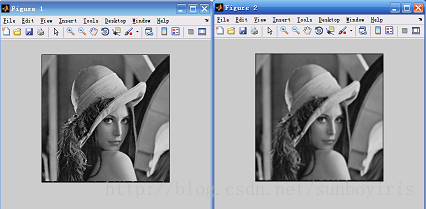
     图像平滑可以减少和抑制图像噪声。

     平均平滑

I = imread('../baby_noise.bmp'); 
figure, imshow(I) 
h = fspecial('average', 3); % 3*3平均模板
I3 = imfilter(I, h, 'corr', 'replicate'); % 相关滤波，重复填充边界
figure, imshow(I3) 
h = fspecial('average', 5) % 5*5平均模板

I5 = imfilter(I, h, 'corr', 'replicate');
figure, imshow(I5) 
h = fspecial('average', 7); % 7*7平均模板
I7 = imfilter(I, h, 'corr', 'replicate');
figure, imshow(I7) 

     高斯平滑

 I = imread('../baby_noise.bmp');
 figure, imshow(I); 

 h3_5 = fspecial('gaussian', 3, 0.5); % sigma=0.5的3*3高斯模板
 I3_5 = imfilter(I, h3_5); % 高斯平滑
 figure, imshow(I3_5); 
 
 h3_8 = fspecial('gaussian', 3, 0.8); % sigma=0.8的3*3高斯模板
 I3_8 = imfilter(I, h3_8);
 figure, imshow(I3_8); 

 h3_18 = fspecial('gaussian', 3, 1.8) % sigma=1.8的3*3高斯模板，接近于平均模板

 I3_18 = imfilter(I, h3_18);
 figure, imshow(I3_18); 

    中值滤波

    

I = imread('../lena_salt.bmp');
imshow(I); 
J=imnoise(I,'salt & pepper');%为图像叠加椒盐噪声
figure, imshow(J); 
w = [1 2 1;2 4 2;1 2 1] / 16;
J1=imfilter(J, w, 'corr', 'replicate'); %高斯平滑
figure, imshow(J1); 
w = [1 1 1;1 1 1;1 1 1] / 9;
J2=imfilter(J, w, 'corr', 'replicate');%平均平滑
figure, imshow(J2); 
J3=medfilt2(J,[3,3]);%中值滤波
figure, imshow(J3);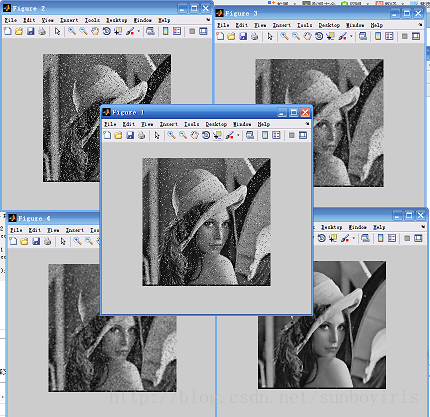

目测 中值滤波效果最好，其为统计排序滤波器，线性平滑滤波器在降噪时不可避免的出现模糊。低于椒盐噪声，中值滤波最好。

    图像锐化

    增强图像灰度跳变部分。锐化的对象是边缘，处理不涉及噪声。

基于一阶导数的增强。

% 基于Robert交叉梯度的图像锐化

I = imread('../bacteria.bmp');
imshow(I); 
I = double(I); % 转换为double型，这样可以保存负值，否则uint8型会把负值截掉
w1 = [-1 0; 0 1]
w2 = [0 -1; 1 0]
G1 =  imfilter(I, w1, 'corr', 'replicate'); % 以重复方式填充边界
G2 =  imfilter(I, w2, 'corr', 'replicate');
G = abs(G1) + abs(G2); % 计算Robert梯度 
figure, imshow(G, []); 
figure, imshow(abs(G1), []);
figure, imshow(abs(G2), []);

基于二阶微分的增强。

% 基于3种拉普拉斯模板的滤波 

I = imread('../bacteria.bmp');
figure, imshow(I);
I = double(I);
w1 = [0 -1 0; -1 4 -1; 0 -1 0]
L1 = imfilter(I, w1, 'corr', 'replicate');
w2 = [-1 -1 -1; -1 8 -1; -1 -1 -1]
L2 = imfilter(I, w2, 'corr', 'replicate');
figure, imshow(abs(L1), []);
figure, imshow(abs(L2), []);
w3 = [1 4 1; 4 -20 4; 1 4 1]
L3 = imfilter(I, w3, 'corr', 'replicate');
figure, imshow(abs(L3), []);

高斯-拉普拉斯变换增强。

LoG算子的锐化
clear all
I = imread('../babyNew.bmp');
figure, imshow(I, []); %得到图5.14（a）
Id = double(I); % 滤波前转化为双精度型

h_log = fspecial('log', 5, 0.5); % 大小为5，sigma=0.5的LoG算子
I_log = imfilter(Id, h_log, 'corr', 'replicate'); 
figure, imshow(uint8(abs(I_log)), []);

h_log = fspecial('log', 5, 2); % 大小为5，sigma=2的LoG算子
I_log = imfilter(Id, h_log, 'corr', 'replicate'); 
figure, imshow(uint8(abs(I_log)), []);