


bokeh是python中一款基于网页的画图工具库,画出的图像以html格式保存。
一个简单的例子:
from bokeh.plotting import figure, output_file, show

output_file("patch.html")

p = figure(plot_width=400, plot_height=400)

# add a patch renderer with an alpha an line width
p.patch([1, 2, 3, 4, 5], [6, 7, 8, 7, 3], alpha=0.5, line_width=2)

show(p)
画出图像后:

代码中有一行为
from bokeh.plotting import figurefigure是一个什么类型的数据?通过查看源代码,发现原来figure是一个函数,返回值为Figure类,Figure类以来自bokeh.models中的Plot类为父类,Figure类继承了Plot类中的各种属性。
from ..models import ColumnDataSource, Plot, Title, Tool, GraphRenderer

class Figure(Plot):
省略...

def figure(**kwargs):
    ''' Create a new :class:`~bokeh.plotting.figure.Figure` for plotting.

    Figure objects have many glyph methods that can be used to draw
    vectorized graphical glyphs:

    .. hlist::
        :columns: 3

{glyph_methods}

    There are also two specialized methods for stacking bars:

    * :func:`~bokeh.plotting.figure.Figure.hbar_stack`
    * :func:`~bokeh.plotting.figure.Figure.vbar_stack`

    And one specialized method for making simple hexbin plots:

    * :func:`~bokeh.plotting.figure.Figure.hexbin`

    In addition to the standard :class:`~bokeh.plotting.figure.Figure`
    property values (e.g. ``plot_width`` or ``sizing_mode``) the following
    additional options can be passed as well:

    .. bokeh-options:: FigureOptions
        :module: bokeh.plotting.figure

    Returns:
       Figure

    '''

    return Figure(**kwargs)
Plotting with Basic Glyphs
Creating Figures
Scatter Markers
画出圆形可以使用circle()方法:
from bokeh.plotting import figure, output_file, show

# output to static HTML file
output_file("line.html")

p = figure(plot_width=400, plot_height=400)

# add a circle renderer with a size, color, and alpha
p.circle([1, 2, 3, 4, 5], [6, 7, 2, 4, 5], size=20, color="navy", alpha=0.5)

# show the results
show(p)
得到的图形为:

同样的,如果要画出方形,可以使用square()方法,参数都是一样,将代码中的circle替换为square即可:
from bokeh.plotting import figure, output_file, show

# output to static HTML file
output_file("square.html")

p = figure(plot_width=400, plot_height=400)

# add a square renderer with a size, color, and alpha
p.square([1, 2, 3, 4, 5], [6, 7, 2, 4, 5], size=20, color="olive", alpha=0.5)

# show the results
show(p)
画出的图形为:

还有许多其它图形函数,其参数也都是一样,x表示x轴的数据,y表示y轴的数据,size表示图形的大小。还有一些参数包含angle——表示角度的大小,radius——表示图形的半径。
详细使用方法见:
https://bokeh.pydata.org/en/latest/docs/reference/plotting.html#bokeh.plotting.figure.Figure.x
以annular_wedge()函数为例:
from bokeh.plotting import figure, output_file, show

# output to static HTML file
output_file("square.html")

p = figure()
x = [61,62,63,64,65]
y = [66,67,68,69,70]

# add a square renderer with a size, color, and alpha
p.annular_wedge(x=x, y=y, inner_radius=0.1, outer_radius=0.3, start_angle=0, end_angle=5, direction='anticlock')

# show the results
show(p)
Line Glyphs
Single Lines
from bokeh.plotting import figure, output_file, show

output_file("line.html")

p = figure(plot_width=400, plot_height=400)

# add a line renderer
p.line([1, 2, 3, 4, 5], [6, 7, 2, 4, 5], line_width=2)

show(p)
Step Lines
from bokeh.plotting import figure, output_file, show

output_file("line.html")

p = figure(plot_width=400, plot_height=400)

# add a steps renderer
p.step([1, 2, 3, 4, 5], [6, 7, 2, 4, 5], line_width=2, mode="center")

show(p)
Multiple Lines
from bokeh.plotting import figure, output_file, show

output_file("patch.html")

p = figure(plot_width=400, plot_height=400)

p.multi_line([[1, 3, 2], [3, 4, 6, 6]], [[2, 1, 4], [4, 7, 8, 5]],
             color=["firebrick", "navy"], alpha=[0.8, 0.3], line_width=4)

show(p)
需要注意的是,第一个list表示x轴的数据,[[1,3,2],[3,4,6,6]]中的两个list代表lines是分离的;第二个list表示y轴的数据。
Missing Points
NaN可以作为line()和multi_line()函数参数的一部分,用该值可以表示不连续点。若x=NaN,则对应的y值将被忽略。
from bokeh.plotting import figure, output_file, show

output_file("line.html")

p = figure(plot_width=400, plot_height=400)

# add a line renderer with a NaN
nan = float('nan')
p.line([1, 2, 3, nan, 3, 5], [6, 7, 2, 4, 4, 5], line_width=2)

show(p)
Bars and Rectangles
Rectangles
from bokeh.plotting import figure, show, output_file

output_file('rectangles.html')

p = figure(plot_width=400, plot_height=400)
p.quad(top=[2, 3, 4], bottom=[1, 2, 3], left=[1, 2, 3],
       right=[1.2, 2.5, 3.7], color="#B3DE69")

show(p)
还有一个例子:
from math import pi
from bokeh.plotting import figure, show, output_file

output_file('rectangles_rotated.html')

p = figure(plot_width=400, plot_height=400)
p.rect(x=[1, 2, 3], y=[1, 2, 3], width=0.2, height=40, color="#CAB2D6",
       angle=pi/3, height_units="screen")

show(p)
Bars
vertical bars:
from bokeh.plotting import figure, show, output_file

output_file('vbar.html')

p = figure(plot_width=400, plot_height=400)
p.vbar(x=[1, 2, 3], width=0.5, bottom=0,
       top=[1.2, 2.5, 3.7], color="firebrick")

show(p)
horizon bars:
from bokeh.plotting import figure, show, output_file

output_file('hbar.html')

p = figure(plot_width=400, plot_height=400)
p.hbar(y=[1, 2, 3], height=0.5, left=0,
       right=[1.2, 2.5, 3.7], color="navy")

show(p)
Hex Tiles
import numpy as np

from bokeh.io import output_file, show
from bokeh.plotting import figure
from bokeh.util.hex import axial_to_cartesian

output_file("hex_coords.py")

q = np.array([0,  0, 0, -1, -1,  1, 1])
r = np.array([0, -1, 1,  0,  1, -1, 0])

p = figure(plot_width=400, plot_height=400, toolbar_location=None)
p.grid.visible = False

p.hex_tile(q, r, size=1, fill_color=["firebrick"]*3 + ["navy"]*4,
           line_color="white", alpha=0.5)

x, y = axial_to_cartesian(q, r, 1, "pointytop")

p.text(x, y, text=["(%d, %d)" % (q,r) for (q, r) in zip(q, r)],
       text_baseline="middle", text_align="center")

show(p)
import numpy as np

from bokeh.io import output_file, show
from bokeh.plotting import figure
from bokeh.transform import linear_cmap
from bokeh.util.hex import hexbin

n = 50000
x = np.random.standard_normal(n)
y = np.random.standard_normal(n)

bins = hexbin(x, y, 0.1)

p = figure(tools="wheel_zoom,reset", match_aspect=True, background_fill_color='#440154')
p.grid.visible = False

p.hex_tile(q="q", r="r", size=0.1, line_color=None, source=bins,
           fill_color=linear_cmap('counts', 'Viridis256', 0, max(bins.counts)))

output_file("hex_tile.html")

show(p)
Patch Glyphs
Single Patches
from bokeh.plotting import figure, output_file, show

output_file("patch.html")

p = figure(plot_width=400, plot_height=400)

# add a patch renderer with an alpha an line width
p.patch([1, 2, 3, 4, 5], [6, 7, 8, 7, 3], alpha=0.5, line_width=2)

show(p)
Multiple Patches
from bokeh.plotting import figure, output_file, show

output_file("patch.html")

p = figure(plot_width=400, plot_height=400)

p.patches([[1, 3, 2], [3, 4, 6, 6]], [[2, 1, 4], [4, 7, 8, 5]],
          color=["firebrick", "navy"], alpha=[0.8, 0.3], line_width=2)

show(p)
Missing Points
from bokeh.plotting import figure, output_file, show

output_file("patch.html")

p = figure(plot_width=400, plot_height=400)

# add a patch renderer with a NaN value
nan = float('nan')
p.patch([1, 2, 3, nan, 4, 5, 6], [6, 7, 5, nan, 7, 3, 6], alpha=0.5, line_width=2)

show(p)
Ovals and Ellipses
from math import pi
from bokeh.plotting import figure, show, output_file

output_file('ovals.html')

p = figure(plot_width=400, plot_height=400)
p.oval(x=[1, 2, 3], y=[1, 2, 3], width=0.2, height=40, color="#CAB2D6",
       angle=pi/3, height_units="screen")

show(p)
from math import pi
from bokeh.plotting import figure, show, output_file

output_file('ellipses.html')

p = figure(plot_width=400, plot_height=400)
p.ellipse(x=[1, 2, 3], y=[1, 2, 3], width=[0.2, 0.3, 0.1], height=0.3,
          angle=pi/3, color="#CAB2D6")

show(p)
Segments and Rays
Sometimes it is useful to be able to draw many individual line segments at once. Bokeh provides the segment() and ray() glyph methods to render these.
from bokeh.plotting import figure, show

p = figure(plot_width=400, plot_height=400)
p.segment(x0=[1, 2, 3], y0=[1, 2, 3], x1=[1.2, 2.4, 3.1],
          y1=[1.2, 2.5, 3.7], color="#F4A582", line_width=3)

show(p)
The ray() function accepts start points x, y with a length (in screen units) and an angle. The default angle_units are "rad" but can also be changed to "deg". To have an “infinite” ray, that always extends to the edge of the plot, specify 0 for the length:
from bokeh.plotting import figure, show

p = figure(plot_width=400, plot_height=400)
p.ray(x=[1, 2, 3], y=[1, 2, 3], length=45, angle=[30, 45, 60],
      angle_units="deg", color="#FB8072", line_width=2)

show(p)
Wedges and Arcs
from bokeh.plotting import figure, show

p = figure(plot_width=400, plot_height=400)
p.arc(x=[1, 2, 3], y=[1, 2, 3], radius=0.1, start_angle=0.4, end_angle=4.8, color="navy")

show(p)
from bokeh.plotting import figure, show

p = figure(plot_width=400, plot_height=400)
p.wedge(x=[1, 2, 3], y=[1, 2, 3], radius=0.2, start_angle=0.4, end_angle=4.8,
        color="firebrick", alpha=0.6, direction="clock")

show(p)
from bokeh.plotting import figure, show

p = figure(plot_width=400, plot_height=400)
p.annular_wedge(x=[1, 2, 3], y=[1, 2, 3], inner_radius=0.1, outer_radius=0.25,
                start_angle=0.4, end_angle=4.8, color="green", alpha=0.6)

show(p)
from bokeh.plotting import figure, show

p = figure(plot_width=400, plot_height=400)
p.annulus(x=[1, 2, 3], y=[1, 2, 3], inner_radius=0.1, outer_radius=0.25,
          color="orange", alpha=0.6)

show(p)
Combining Multiple Glyphs
from bokeh.plotting import figure, output_file, show

x = [1, 2, 3, 4, 5]
y = [6, 7, 8, 7, 3]

output_file("multiple.html")

p = figure(plot_width=400, plot_height=400)

# add both a line and circles on the same plot
p.line(x, y, line_width=2)
p.circle(x, y, fill_color="white", size=8)

show(p)
Setting Ranges
两种方法设置range:
1.可以通过从bokeh.models中导入Range1d(x,y)对象来实现:
By default, Bokeh will attempt to automatically set the data bounds of plots to fit snugly around the data. Sometimes you may need to set a plot’s range explicitly. This can be accomplished by setting the x_range or y_range properties using a Range1dobject that gives the start and end points of the range you want:
p.x_range = Range1d(0, 100)2.在figure()里直接调用x_range()和y_range():
As a convenience, the figure() function can also accept tuples of (start, end) as values for the x_range or y_range parameters.
看一个例子:
from bokeh.plotting import figure, output_file, show
from bokeh.models import Range1d

output_file("title.html")

# create a new plot with a range set with a tuple
p = figure(plot_width=400, plot_height=400, x_range=(0, 20))

# set a range using a Range1d
p.y_range = Range1d(0, 15)

p.circle([1, 2, 3, 4, 5], [2, 5, 8, 2, 7], size=10)

show(p)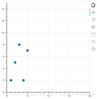
Specifying Axis Types
Categorical Axes
上面的所有例子中,x和y轴都是数字,有些时候希望坐标轴显示的是字符,可以使用如下方法:
from bokeh.plotting import figure, output_file, show

factors = ["a", "b", "c", "d", "e", "f", "g", "h"]
x = [50, 40, 65, 10, 25, 37, 80, 60]

output_file("categorical.html")

p = figure(y_range=factors)

p.circle(x, factors, size=15, fill_color="orange", line_color="green", line_width=3)

show(p)
此时,y轴是factors:

Log Scale Axes
from bokeh.plotting import figure, output_file, show

x = [0.1, 0.5, 1.0, 1.5, 2.0, 2.5, 3.0]
y = [10**xx for xx in x]

output_file("log.html")

# create a new plot with a log axis type
p = figure(plot_width=400, plot_height=400, y_axis_type="log")

p.line(x, y, line_width=2)
p.circle(x, y, fill_color="white", size=8)

show(p)
Twin Axes
from numpy import pi, arange, sin, linspace

from bokeh.plotting import output_file, figure, show
from bokeh.models import LinearAxis, Range1d

x = arange(-2*pi, 2*pi, 0.1)
y = sin(x)
y2 = linspace(0, 100, len(y))

output_file("twin_axis.html")

p = figure(x_range=(-6.5, 6.5), y_range=(-1.1, 1.1))

p.circle(x, y, color="red")

p.extra_y_ranges = {"foo": Range1d(start=0, end=100)}
p.circle(x, y2, color="blue", y_range_name="foo")
p.add_layout(LinearAxis(y_range_name="foo"), 'left')

show(p)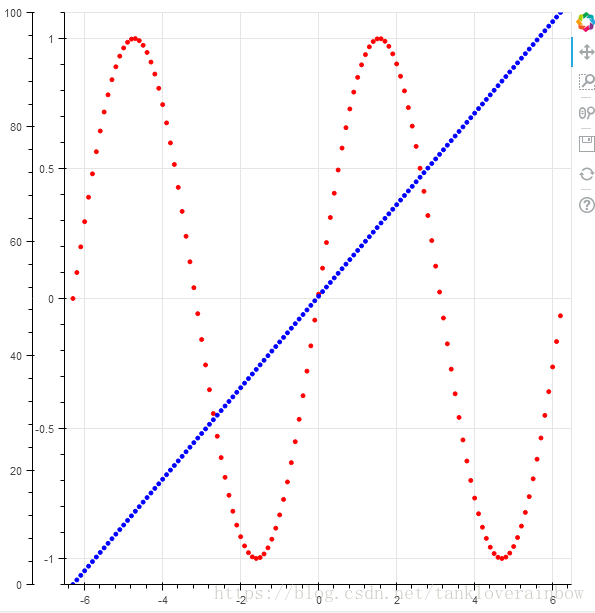


 1647
1647

 被折叠的 条评论
为什么被折叠?
被折叠的 条评论
为什么被折叠?
 到【灌水乐园】发言


