卷积神经网络必备基础

卷积神经网络（Convolutional Neural Network,  CNN）

传统的全连接神经网络并不适用于图像处理，这是因为：每个像素点都是一个输入特征，随着层数的增加，参数以指数级增长，而图片的像素点往往非常多，导致参数的规模非常巨大。

例如：

• 32x32的图片：仅仅输入层，就有32x32x3（三原色） = 3072个特征
• 200x200的图片：仅仅输入层，就有200x200x3（三原色） = 120000个特征

仅仅特征就有这么多，其后的隐藏层，对应的权重参数的数量是：（特征数）x (隐藏层结点数)，可以想象这个参数的规模。

卷积（Convolution）

本文只解释卷积的具体操作，不讨论卷积的数学定义。如下所示，对于左上角的原始矩阵数据，我们使用一个卷积核（Convolution Kernel，也成为过滤器filter）的3x3小方阵，依次和原始矩阵数据中的每一个3x3的子方阵数据做“相乘+求和”的操作。

以图中为例

• 绿色的两个区域的卷积计算过程见图片右上角，得到计算结果“-8”，即完成了一次卷积运算。
• 下一次卷积运算，是将第一个3x3子方阵向右平移一个单位，得到第二个3x3子方阵，将其和卷积核相乘再求和，得到结果依然是-8。
• 向右平移到最后一个3x3子方阵之后，回到矩阵最左边，再向下平移一个单位，得到3x3子方阵，将其和卷积核相乘再求和，得到结果依然是-8。
• 按照这个顺序平移下去，直到最后一个3x3子方阵的卷积运算完成，得到结果为一个5x5矩阵

填充零（Zero Padding）

通过前面的例子可以看出，在对一张原始图片像素数据执行卷积计算后，得到的输出数据尺寸往往会略小于原始数据的尺寸（例子中7x7的矩阵经过计算后得到一个较小的5x5矩阵）。如果希望输出相同尺寸的数据，则可以在原始矩阵外围填充零，然后再进行卷积计算。注意：一般这个操作会对图片的上下左右对称填充，如下所示

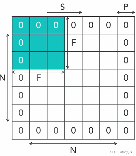
假设：N为原始图片大小，F为卷积核（过滤器）大小，S为移动步长，P为填充零的（P是上下左右对称填充），则卷积操作后，得到的图片大小为：。

汇聚（Pooling，也有翻译为池化）

在神经网络介绍中，我们已经介绍了常用的汇聚层算法有：取最大值，取平均值，取线性组合等。一般最常用的就是前两种，分别称为最大汇聚（Max Pooling）和平均汇聚（Average Pooling）。

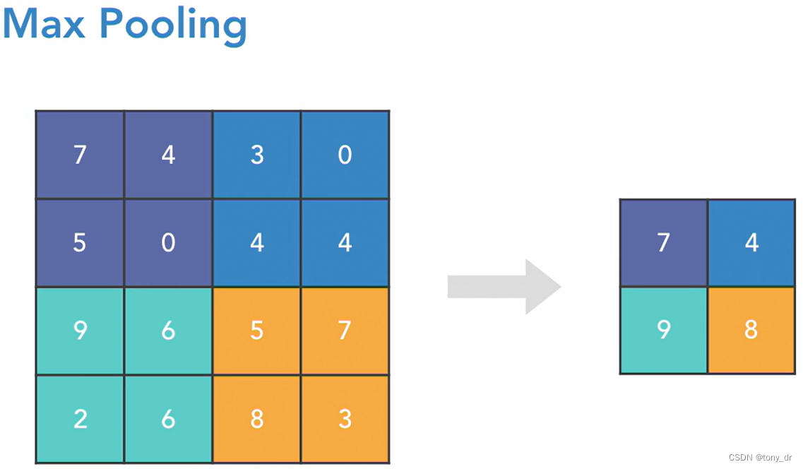
最大汇聚

确定一个过滤器的大小，对原数据中同样大小区域的数据取最大值，作为结果。如下所示，对于原始的4x4数据，确定过滤器大小为2x2，则对4x4数据上的每一个2x2区域选一个最大值。这样的区域一共有4个（注意：每一个划分出来的2x2区域是不重叠的）。依次取出最大值7、4、9、8，得到了右边的汇聚结果。

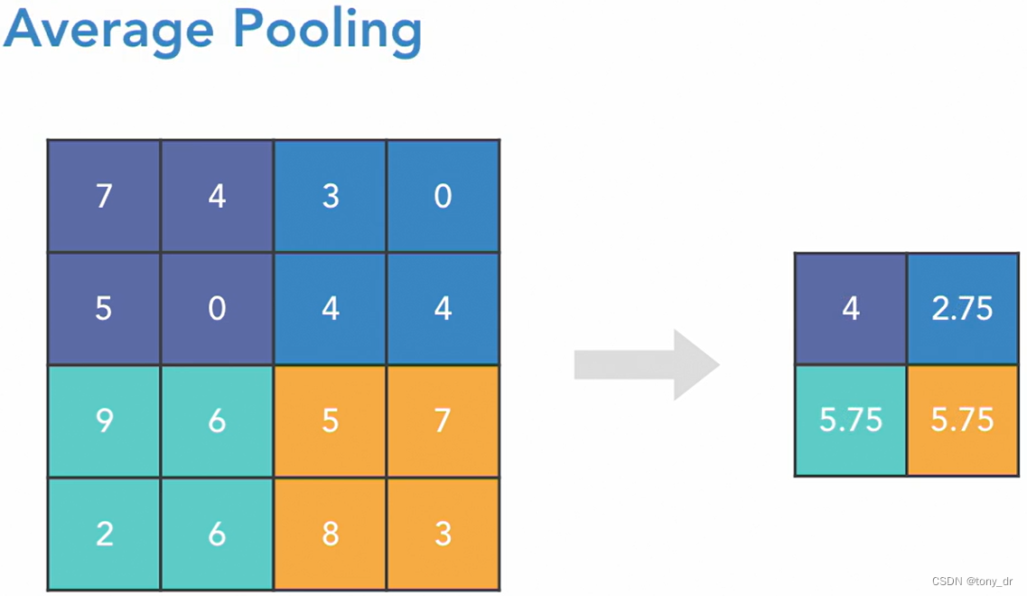
平均汇聚

和最大汇聚的区别是：对每一区域取平均值作为结果

汇聚的作用是什么？

• 以非线性的方式降低采样，减少参数和计算量
• 降低了过拟合（Overfitting）的机率
• 降低原始数据的大小，意味着损失了一些信息，因此一般会增加过滤器的个数

各种汇聚中，最大汇聚是最流行的，因为

• 它可以提升一个图片在某个区域的显著特征
• 在降低采样的时候，它能保留图片中最具有特征的部分

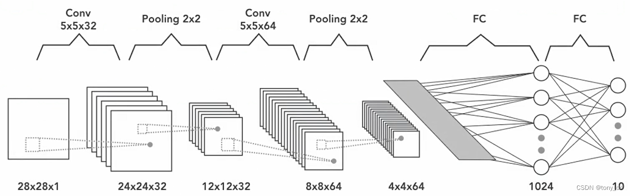
在卷积神经网络必备基础中，我们使用了传统的FNN模型解决了MNIST问题。下图是这个问题的CNN处理模型，下一节将用程序来实现这个模型。

使用Keras实现CNN

1. 导入Python的包

注意：在层的导入中，我们导入了卷积层Conv2D，最大汇聚层MaxPooling2D，平铺层Flatten（将矩阵数据平铺为向量），全连接层Dense

from keras.datasets import mnist
from keras.utils import to_categorical
from keras.models import Sequential
from keras.layers import Conv2D, MaxPooling2D, Flatten, Dense

import matplotlib.pyplot as plt

# Allow view plots in the notebook, '%' is a magic usage for python for special
%matplotlib inline

2. 加载数据

和神经网络必备基础中一样

(X_train_raw, y_train_raw), (X_test_raw, y_test_raw) = mnist.load_data()
print(X_train_raw.shape, X_test_raw.shape)
print(y_train_raw.shape, y_test_raw.shape)

3. 预处理训练数据

注意：对图像数据进行卷积操作，需要将数据reshape为3维，即（长，宽，颜色），因为是黑白图片，所以“颜色”这个维度取1，如果是彩色，则“颜色”这个维度取3

# suppose we don't know the data shape of the raw loaded MNIST data
# , we must make sure the data shape is what we wanted
X_train = X_train_raw.reshape(60000,28,28,1)
X_test = X_test_raw.reshape(10000,28,28,1)

# centered the data value, which is divided by 255 (each pixel value is 0~255)
X_train = X_train.astype('float32') / 255.0
X_test = X_test.astype('float32') / 255.0
print(X_train.shape, X_test.shape)

4. 预处理测试数据

和神经网络必备基础中一样，我们将标签扩张为一个由若干0和1组成的向量。

# convert each class value to a vector with value of 0 or 1
# i.e. if class vector, then it will be a matrix with value of 0 or 1
# e.g. for 0~9, 10 classes in total, if value is 5, then it will be
#      coverted to [0,0,0,0,0,1,0,0,0,0]
y_train = to_categorical(y_train_raw, NUM_CLASSES)
y_test = to_categorical(y_test_raw, NUM_CLASSES)
print(y_train.shape, y_test.shape)
print(y_train[0])

5. 创建和编译模型

cnn = Sequential()
cnn.add(Conv2D(32, kernel_size=(5,5), input_shape=(28,28,1), padding='same',activation='relu'))
cnn.add(MaxPooling2D())
cnn.add(Conv2D(64, kernel_size=(5,5), padding='same',activation='relu'))
cnn.add(MaxPooling2D())
cnn.add(Flatten())
cnn.add(Dense(1024, activation='relu'))
cnn.add(Dense(10, activation='softmax'))

cnn.compile(optimizer='adam', loss='categorical_crossentropy', metrics=['accuracy'])
print(cnn.summary())

summary()输出如下：

Model: "sequential_3"
_________________________________________________________________
 Layer (type)                Output Shape              Param #   
=================================================================
 conv2d_5 (Conv2D)           (None, 28, 28, 32)        832       
                                                                 
 max_pooling2d_5 (MaxPoolin  (None, 14, 14, 32)        0         
 g2D)                                                            
                                                                 
 conv2d_6 (Conv2D)           (None, 14, 14, 64)        51264     
                                                                 
 max_pooling2d_6 (MaxPoolin  (None, 7, 7, 64)          0         
 g2D)                                                            
                                                                 
 flatten_2 (Flatten)         (None, 3136)              0         
                                                                 
 dense_4 (Dense)             (None, 1024)              3212288   
                                                                 
 dense_5 (Dense)             (None, 10)                10250     
                                                                 
=================================================================
Total params: 3274634 (12.49 MB)
Trainable params: 3274634 (12.49 MB)
Non-trainable params: 0 (0.00 Byte)
_________________________________________________________________
None

关于参数个数的说明：

• 对于汇聚层，因为是对原数据取最大值，所以不需要参数
• 对于卷积层，参数即卷积核中的参数，外加每一个新图片数据对应的一个偏好参数，例如
  • 对于conv2d_5层：每个卷积核有5x5=25个参数，由1个输入图片产生32个输出图片，于是由1x32个卷积核，外加32个偏好，总共有5x5x1x32+32 = 832个参数
  • 对于conv2d_6层：同理，总共有5x5x32x64+64 = 51264个参数
• 对于平铺层，只是将数据展开，所以也不需要参数
• 对于全连接层dense_4：3136(7x7x64) x 1024+1024=3212288
• 对于全连接层dense_5：1024x10_10=10250

6. 训练和评价模型

这个模型训练时间比较长，是因为我们在卷积层使用了较多的特征提取：第一次卷积操作从一张图中提取了32种不同的特征，第二次卷积操作从32张图种提取了更多的特征。注意到，如果图片像素增加了，只要卷积核和特征图片的种类不变，上述模型的参数是不会增加的。

history_cnn = cnn.fit(X_train, y_train, epochs=2, verbose=1, validation_data=(X_test, y_test))

输出如下：

Epoch 1/2
1875/1875 [==============================] - 227s 121ms/step - loss: 0.0980 - accuracy: 0.9693 - val_loss: 0.0304 - val_accuracy: 0.9895
Epoch 2/2
1875/1875 [==============================] - 221s 118ms/step - loss: 0.0362 - accuracy: 0.9888 - val_loss: 0.0244 - val_accuracy: 0.9918

可以看到，每个epoch训练时间接近4分钟。

使用evaluate()评价模型

score = cnn.evaluate(X_test, y_test)
print(score)

得到输出如下：

313/313 [==============================] - 9s 28ms/step - loss: 0.0244 - accuracy: 0.9918
[0.024433128535747528, 0.9918000102043152]

和神经网络必备基础种的FNN相比，这里我们得到了更高的准确度：99.18%

CNN的增强

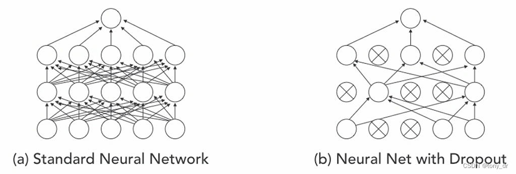
丢弃（Dropout）

• 以p为概率、随机去掉一些训练层中的神经元（结点）
• 目的：防止过拟合，只能用于训练数据

图像增强（image augmentation）

从训练集中取出图片数据，然后对其进行某些操作，从而：

• 得到更多的图片用于模型训练
• 通过操作后得到的新图片，使得模型更加健壮

关于这部分的细节，可以参考这篇博文：（数据）图像预处理——image augmentation图像增广之cutout、Mixup、CutMix方法及其实现_cutmix代码实现-CSDN博客

用Keras可以实现图像增强，程序如下

import numpy as np
from keras.preprocessing.image import ImageDataGenerator, array_to_img, img_to_array, load_img
from keras.applications.inception_v3 import preprocess_input

train_datagen = ImageDataGenerator(
    preprocessing_function=preprocess_input,
    width_shift_range=0.2,
    height_shift_range=0.2,
    shear_range=0.2,
    zoom_range=0.2,
    horizontal_flip=True)

train_generator = train_datagen.flow_from_directory('Colab Notebooks/images/sample_train/',
                                  target_size=(150, 150),
                                  save_to_dir='Colab Notebooks/images/sample_confirm/')

可以看到，Keras提供了ImageDataGenerator()这个类实现了这一功能：在'Colab Notebooks/images/sample_train/'这个路径下预先存放了几张原始图片，然后在'Colab Notebooks/images/sample_confirm/'路径下根据原始团片产生了很多新的图片。

这段程序不详解了，有兴趣可以自己查阅手册研究。

ImageNet介绍

什么是ImageNet

• 一个很容易访问的大规模图片数据库
• 起始于2009年
• 基于WordNet架构
• 每一个概念有多个同义词集合(synset, or synonym set)描述，例如对于Continental glacier(大陆冰川)有以下同义词集：Geological formation | ice mass | glacier | continental glacier
• 当前，每一个同义词集大约有1000张图片

 ImageNet网址：https://image-net.org/

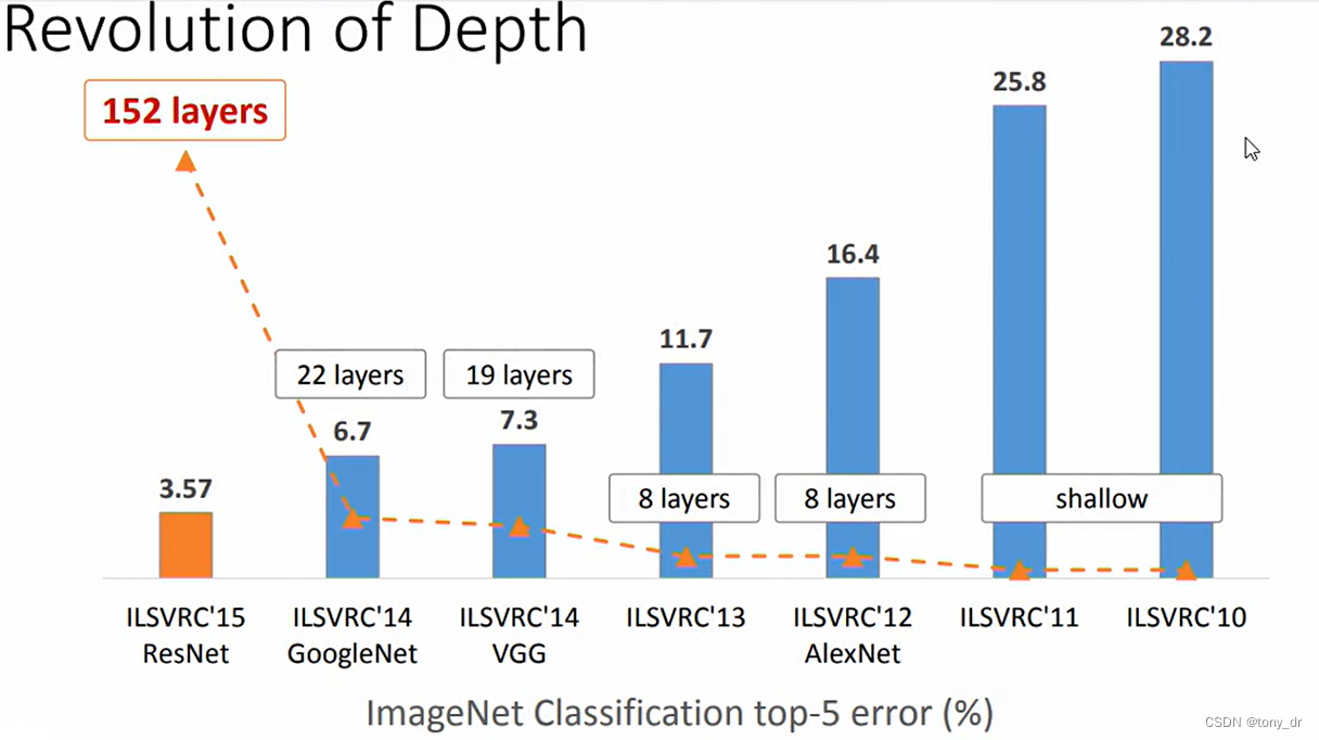
ImageNet挑战赛（ImageNet Challenge）

• 每年一次的竞赛：区分几千张照片，并将其划分到1000个类别中
• 全称ImageNet Large Scale Visual Recognition Challenge (ILSVRC)

下图反映了从10年到15年参加ILSVRC的优秀模型的深度（层数）变化，可以看到深度是在逐渐降低的。

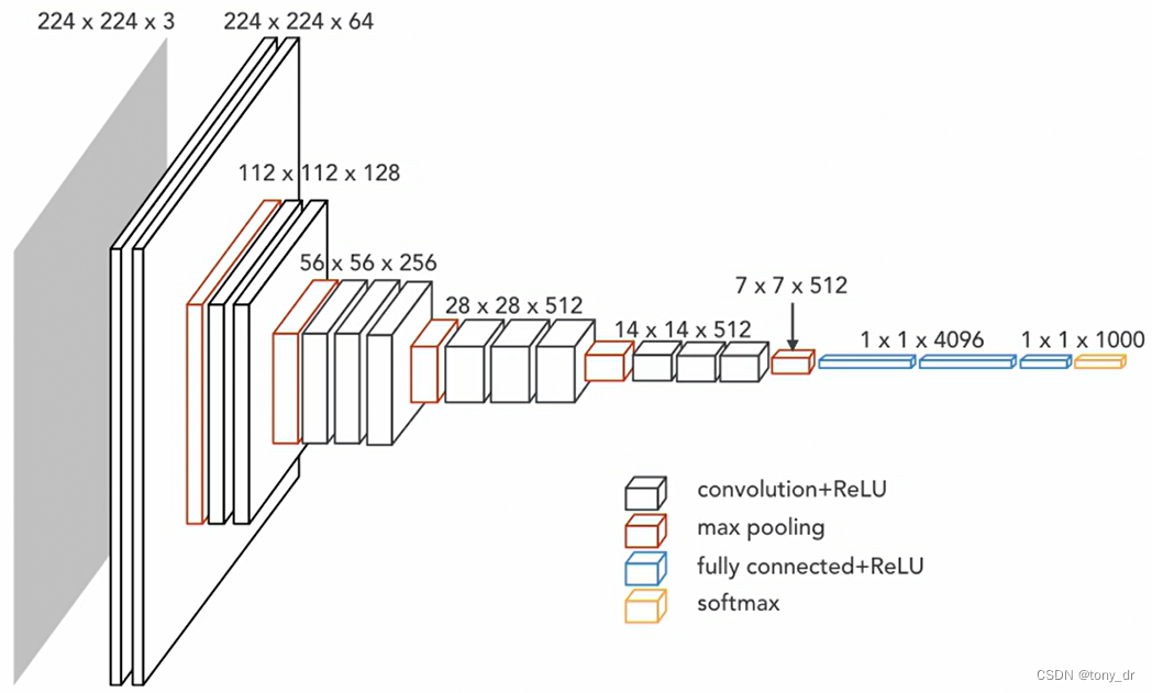
VGG模型

VGG模型是一种深度卷积神经网络（CNN），由牛津大学的Visual Geometry Group（Oxford VGG）提出，该模型在2014年的ILSVRC（ImageNet大规模视觉识别挑战赛）中获得了第二名。VGG模型在多个迁移学习任务中的表现优于其他模型，并且从图像中提取CNN特征时，VGG模型是首选算法。

VGG16模型的示意图如下：

Keras同样也支持了VGG模型，程序如下：

import numpy as np
from keras.applications import vgg16
from keras.preprocessing import image

model = vgg16.VGG16(weights='imagenet')
# VGG16 model requires a image size of 224x224
img = image.load_img('Colab Notebooks/images/sample_train/cats/cat_02.jpeg',
                     target_size=(224,224))
img

#convet to numpy array
arr = image.img_to_array(img)
arr.shape

# expand dimension, as 1 dimension is batch, or else predict() will report error
#  "convolution input must be 4-dimensional:"
arr = np.expand_dims(arr, axis=0)
arr.shape

# preprocessing
arr = vgg16.preprocess_input(arr)
arr

# predict
pred = model.predict(arr)
# shows probilites in 1000 categories, as vgg model has 1000 categories
pred

# predications for top5
vgg16.decode_predictions(pred, top=5)

上述程序对我们存放的一张猫的图片：'Colab Notebooks/images/sample_train/cats/cat_02.jpeg'，使用vgg16直接进行预测。程序输出如下：

[[('n02123045', 'tabby', 0.6933489),
  ('n02123159', 'tiger_cat', 0.13225932),
  ('n02124075', 'Egyptian_cat', 0.098001406),
  ('n02123394', 'Persian_cat', 0.009920092),
  ('n02883205', 'bow_tie', 0.0063082646)]]

可以看到，模型预测出来的结果中，具有最大概率的是'tabby'(斑猫)。