算法导论第三版第2章习题答案

最新推荐文章于 2023-07-13 13:22:58 发布

时时处处皆修行

最新推荐文章于 2023-07-13 13:22:58 发布

阅读量7.3k

点赞数 5

分类专栏： Algorithm 文章标签：算法导论 python

本文链接：https://blog.csdn.net/davidwang9527/article/details/109287003

版权

Algorithm 专栏收录该内容

8 篇文章 14 订阅

订阅专栏

2020/10/27: 增加伪代码相应的Python实现代码。
2020/11/13:修订第2节第3题的bug。
参考文献：https://ita.skanev.com/

2 Getting Started

2.1 Insertion sort

1.Using Figure 2.2 as a model, illustrate the operation of INSERTION-SORT on the array A=<31; 41; 59; 26; 41; 58>.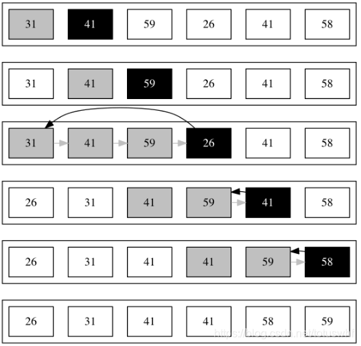

2.Rewrite the Insertion-Sort procedure to sort into nonincreasing instead of non-decreasing order.

The only thing we need to do is flipping the comparison:

for j = 2 to A.length
    key = A[j]
    i = j - 1
    while i > 0 and A[i] < key
        A[i + 1] = A[i]
        i = i - 1
    A[i + 1] = key

Python implementation:

def insertion_sort_desc(A):
    for j in range(1,len(A)):
        key = A[j]
        i = j - 1
        while i >= 0 and A[i] < key :
            A[i + 1] = A[i]
            i = i - 1
        A[i + 1] = key
    
    return A

A = [3, 4 , 2, 1]
print(insertion_sort_desc(A))

3.Consider the searching problem:

Input: A sequence of n numbers $A=<a_1,a_2,a_n>$ and a value ν.

Output: And index i such that ν=A[i] or the special value NIL if ν does not appear in A

Write the pseudocode for linear search, which scans through the sequence, looking for ν. Using a loop invariant, prove that your algorithm is correct. Make sure that your loop invariant fulfills the three necessary properties.

The pseudocode looks like this:

SEARCH(A, v):
  for i = 1 to A.length
      if A[i] == v
          return i
  return NIL

Python Implementation:

def search_in_array(A, v):
    for i in range(len(A)):
        if v == A[i]:
            return i
    
    return None

print(search_in_array([1,2,3,4],2))
print(search_in_array([1,2,3,4],5))

I'm going to state the loop invariant as:

At the start of each iteration of the for loop, the subarray A[1..i−1] consists of elements that are different than ν.

Here are three properties:

Initialization

Initially the subarray is the empty array, so proving it is trivial.

Maintenance

On each step, we know that A[1..i−1] does not contain ν. We compare it with A[i]. If they are the same, we return i, which is a correct result. Otherwise, we continue to the next step. We have already ensured that A[A..i−1] does not contain ν and that A[i] is different from ν, so this step preserves the invariant.

Termination

The loop terminates when i>A.length. Since i increases by 1 and i>A.length, we know that all the elements in A have been checked and it has been found that ν is not among them. Thus, we return NIL.

4.Consider the problem of adding two n-bit binary integers, stored in two n-element arrays A and B. The sum of the two integers should be stored in binary form in an (n + 1)-element array C. State the problem formally and write pseudocode for adding the two integers.

The formal statement:

Input: An array of booleans $A = \langle a_1, a_2, \ldots, a_n \rangle$ , an array of booleans $B = \langle b_1, b_2, \ldots, b_n \rangle$ , each representing an integer stored in binary format (each digit is a number, either 0 or 1, least-significant digit first) and each of length n.

Output: An array $C = \langle c_1, c_2, \ldots, c_{n+1} \rangle$ that such that C' = A' + B', where A', B' and C' are the integers, represented by A, B and C.

Here is the pseudocode:

ADD-BINARY(A, B):
  C = new integer[A.length + 1]

  carry = 0
  for i = 1 to A.length
      C[i] = (A[i] + B[i] + carry) % 2  // remainder
      carry = (A[i] + B[i] + carry) / 2 // quotient
  C[i] = carry

  return C

Python implementation:

def add_binary(A , B):
    c = [2]*(len(A) + 1)

    carry = 0 
    for i in range(len(A)):
        c[i] = (A[i] + B[i] + carry) % 2  #remainder
        carry = (A[i] + B[i] + carry) // 2 #quotient

    c[i + 1] = carry

    return c

A = [1,1,0,1]
B = [1,1,0,1]
print(add_binary(A , B))

2.2 Analyzing algorithms

1.Express the function $n^3/1000 - 100n^2 - 100n +3$ in terms of Θ-notation

$\Theta(n^3)$

2.Consider sorting n numbers in an array A by first finding the smallest element of A and exchanging it with the element in A[1]. Then find the second smallest element of A, and exchange it with A[2]. Continue in this manner for the first n−1 elements of A. Write pseudocode for this algorithm, which is known as selection sort. What loop invariants does this algorithm maintain? Why does it need to run for only the first n−1 elements, rather than for all n elements? Give the best-case and the worst-case running times of selection sort in Θ-notation.

Pseudocode

SELECTION-SORT(A):
  for i = 1 to A.length - 1
      min = i
      for j = i + 1 to A.length
          if A[j] < A[min]
              min = j
      temp = A[i]
      A[i] = A[min]
      A[min] = temp

Python Implementation:

def selection_sort(lst):
    for i in range(0, len(lst)-1):
        min_index = i
        for j in range(i + 1, len(lst)):
            if lst[j] < lst[min_index]:
                min_index = j
        temp = lst[i]
        lst[i] = lst[min_index]
        lst[min_index]=temp
    return lst      

print(selection_sort([4,3,2,1]))

Loop invariants:

Initialization

Initially the subarray is the empty array, so proving it is trivial.

Maintenance

At the start of each iteration of the outer for loop, the subarray A[1..i−1] contains the smallest i−1 elements of the array, sorted in nondecreasing order. And at the start of each iteration of the inner for loop, A[min] is the smallest number in the subarray A[i..j−1].

Termination

The loop terminates when i>A.length-1. We know that A[i..A.length-1] contains the smallest .length-1 elements of the array, which means the array has been well sorted.

Why n−1 elements?

In the final step, the algorithm will be left with two elements to compare. It will store the smaller one in A[n−1] and leave the larger in A[n]. The final one will be the largest element of the array since all the previous iteration would have sorted all but the last two elements (the outer loop invariant). If we do it n times, we will end up with a redundant step that sorts a single-element subarray.

Running times

In the best-case time (the array is sorted), the body of the if is never invoked. The number of operations (counting the comparison as one operation) is:

$\left ( n - 1 \right )\left ( \frac{n + 2}{2}+4 \right )$

In the worst-case time (the array is reversed), the body of the if is invoked on every occasion, which doubles the number of steps in the inner loop, that is:

(n−1)(n+6)

Both are clearly $\Theta(n^2)$ .

3.Consider linear search again (see exercise 2.1-3). How many elements of the input sequence need to be checked on the average, assuming that the element being searched for is equally likely to be any element in the array? How about the worst case? What are the average-case and worst-case running times of linear search in Θ-notation? Justify your answers.

If the element is present in the sequence, half of the elements are likely to be checked before it is found in the average case. In the worst case, all of them will be checked. That is, n/2 checks for the average case and n for the worst case. Both of them are Θ(n).

4.How can we modify almost any algorithm to have a good best-case running time?

We can modify it to handle the best-case efficiently. For example, if we modify insertion-sort to check if the array is sorted and just return it, the best-case running time will be Θ(n).

2.3 Designing algorithms

1.Using Figure 2.4 as a model, illustrate the operation of merge sort on the array A=〈3,41,52,26,38,57,9,49〉.

]

2.Rewrite the MERGE procedure so that it does not use sentinels, instead stopping once either array L or R has had all its elements copied back to A and then copying the remainder of the other array back into A.

MERGE(A, p, q, r)
  n1 = q - p + 1
  n2 = r - q
  let L[1..n₁] and R[1..n₂] be new arrays
  for i = 1 to n₁
      L[i] = A[p + i - 1]
  for j = 1 to n₂
      R[j] = A[q + j]
  i = 1
  j = 1
  for k = p to r
      if i > n₁
          A[k] = R[j]
          j = j + 1
      else if j > n₂
          A[k] = L[i]
          i = i + 1
      else if L[i] ≤ R[j]
          A[k] = L[i]
          i = i + 1
      else
          A[k] = R[j]
          j = j + 1

Python Implementation:

def merge_without_guard(A, p, q, r):
    n1 = q - p + 1
    n2 = r - q
    L = [0]*n1
    R = [0]*n2
    
    L = A[p : p + n1]
    R = A[q + 1 : q + n2 +1]

    # Merge the temp arrays back into A[p..r] 
    i = 0     # Initial index of first subarray 
    j = 0     # Initial index of second subarray 
    
    for k in range(p , r + 1):
        if i == n1:
            A[k] = R[j]
            j += 1
        elif j == n2:
            A[k] = L[i]
            i += 1
        elif L[i] <= R[j]:
            A[k] = L[i]
            i += 1
        else:
            A[k] = R[j]
            j += 1
    return A

def merge_sort_without_guard(A, p, r):
    if p < r:
        q = (p + r ) // 2
        merge_sort_without_guard(A, p , q)
        merge_sort_without_guard(A, q + 1, r)
        merge_without_guard(A, p , q, r)
    return A

A =[1,3,2,4]
print(merge_sort_without_guard(A, 0, 3))

A =[12,11,13,5,7,6]
print(merge_sort_without_guard(A, 0, 5))

A =[3,2,1,4,6,5]
print(merge_sort_without_guard(A, 0, 5))

3.Use mathematical induction to show that when n is an exact power of 2, the solution of the recurrence

$T(n)=\begin{cases} 2\quad if n=2 \\ 2T(n/2) +n \quad if n=2^k,for\quad k >1 \end{cases}$

is T(n)=nlgn

4.We can express insertion sort as a recursive procedure as follows. In order to sort A[1..n], we recursively sort A[1..n−1] and then insert A[n] into the sorted array A[1..n−1]. Write a recurrence for the running time of this recursive version of insertion sort.

The recurrence is

$T(n)=\begin{cases} \Theta(1)\quad if n=1 \\ T(n-1) + C(n-1) \quad otherwise \end{cases}$

where C(n) is the time to insert an element in a sorted array of n elements.

5.Referring back to the searching problem (see Exercise 2.1-3), observe that if the sequence A is sorted, we can check the midpoint of the sequence against ν and eliminate half of the sequence from further consideration. The binary search algorithm repeats this procedure, halving the size of the remaining portion of the sequence each time. Write pseudocode, either iterative or recursive, for binary search. Argue that the worst-case running time of binary search is Θ(lgn).

BINARY-SEARCH(A, v):
  low = 1
  high = A.length

  while low <= high
      mid = (low + high) / 2
      if A[mid] == v
          return mid
      if A[mid] < v
          low = mid + 1
      else
          high = mid - 1

  return NIL

Python Implementation:

def binary_search(A, v):
    low = 0
    high = len(A)

    while(low < high):
        mid = (low + high) // 2
        
        if A[mid] == v :
            return mid
        elif A[mid] < v:
            low = mid + 1
        else:
            high = mid

    return -1

print(binary_search([1,2,3,4],2))
print(binary_search([1,2,3,4],5))

The argument is fairly straightforward and I will make it brief:

T(n+1)=T(n/2)+c

This is the recurrence shown in the chapter text, and we know, that this is logarithmic time.

6.Observe that the while loop line 5-7 of the INSERTION-SORT procedure in Section 2.1 uses a linear search to scan (backward) through the sorted subarray A[i..j−1]. Can we use a binary search (see Exercise 2.3-5) instead to improve the overall worst-case running time of insertion sort to Θ(nlgn)?

No. Even if it finds the position in logarithmic time, it still needs to shift all elements after it to the right, which is linear in the worst case. It will perform the same number of swaps, although it would reduce the number of comparisons.

7.★ Describe a Θ(nlgn)-time algorithm that, given a set S of n integers and another integer x, determines whether or not there exists two elements of S whose sum is exactly x.

First we sort S. Afterwards, we iterate it and for each element i we perform a binary search to see if there is an element equal to x−i. If one is found, the algorithm returns true. Otherwise, it returns false.

We iterate n elements and perform binary search for each on in an n-sized array, which leads to Θ(nlgn)-time. If we sort first (with merge sort) it will introduce another Θ(nlgn) time, that would change the constant in the final algorithm, but not the asymptotic time.

PAIR-EXISTS(S, x):
  A = MERGE-SORT(S)

  for i = 1 to S.length
      if BINARY-SEARCH(A, x - S[i]) != NIL
          return true

  return false

Python Implementation:


def pair_exists(S,x):
    A = merge_sort_without_guard(S, 0, len(S)-1)
    for i in range(len(S)):
        if binary_search(A, x-S[i]) != -1:
            return True
    
    return False

S = [3,2,1,4,6,5]
print(pair_exists(S,7))
print(pair_exists(S,20))

Note:This is the same as question 1 in leetcode, which recommend a O(n) algorithm.

Problems

2-1 Although merge sort runs in Θ(lgn) worst-case time and insertion sort runs in $\Theta(n^2)$ worst-case time, the constant factors in insertion sort can make it faster in practice for small problem sizes on many machines. Thus, it makes sense to coarsen the leaves of the recursion by using insertion sort within merge sort when subproblems become sufficiently small. Consider a modification to merge sort in which n/k sublists of length k are sorted using insertion sort and then merged using the standard merging mechanism, where k is a value to be determined.

Show that insertion sort can sort the n/k sublists, each of length k, in Θ(nk) worst-case time.
Show how to merge the sublists in Θ(nlg(n/k)) worst-case time.
Given that the modified algorithm runs in Θ(nk+nlg(n/k)) worst-case time, what is the largest value of k as a function of n for which the modified algorithm has the same running time as standard merge sort, in terms of Θ-notation?
How should we choose k in practice?

1. Sorting sublists
This is simple enough. We know that sorting each list takes $ak^2+bk+c$ for some constants a, b and c. We have n/k of those, thus:

$\frac{n}{k}(ak^2 + bk + c) = ank + bn + \frac{cn}{k} = \Theta(nk)$

2. Merging sublists

This is a bit trickier. Sorting a sublists of length k each takes:

$T(a) = \begin{cases} 0 & \text{if } a = 1, \\ 2T(a/2) + ak & \text{if } a = 2^p, \text{if } p > 0. \end{cases}$

This makes sense, since merging one sublist is trivial and merging a sublists means dividing them into two groups of $\frac{a}{2}$ lists, merging each group recursively and then combining the results in $ak$ steps. Since there're two arrays, each of length $\frac{a}{2}k$ .

I don't know the master theorem yet, but it seems to me that the recurrence is actually $ak\lg{a}$ . Let's try to prove this via induction:

Base. Simple as ever:

$T(1) = 1k\lg1 = k \cdot 0 = 0$

Step. We assume that $T(a) = ak\lg{a}$ and we calculate T(2a):

$\begin{align*} T(2a) &= 2T(a) + 2ak = 2(T(a) + ak) = 2(ak\lg{a} + ak) = \\ &= 2ak(\lg{a} + 1) = 2ak(\lg{a} + \lg{2}) = 2ak\lg(2a) \end{align*}$

This proves it. Now if we substitute the number of sublists n/k for a:

$T(n/k) = \frac{n}{k}k\lg{\frac{n}{k}} = n\lg(n/k)$

While this is exact only when n/k is a power of 2, it tells us that the overall time complexity of the merge is Θ(nlg(n/k)).

3. The largest value of k

The largest value is k=lgn. If we substitute, we get:

$\Theta(n\lg{n} + n\lg{\frac{n}{\lg{n}}}) = \Theta(n\lg{n})$

If k=f(n)>lgn, the complexity will be Θ(nf(n)), which is larger running time than merge sort.

4. The value of k in practice

It's constant factors, so we just figure out when insertion sort beats merge sort, exactly as we did in exercise 1.2.2, and pick that number for k.

2-2 Bubblesort is popular, but inefficient, sorting algorithm. It works by repeatedly swapping adjancent elements that are out of order.
BUBBLESORT(A)
  for i to A.length - 1
      for j = A.length downto i + 1
          if A[j] < A[j - 1]
              exchange A[j] with A[j - 1]
Let A′ denote the output of BUBBLESORT(A). To prove that BUBBLESORT is correct, we need to prove that it terminates and that
A′[1]≤A′[2]≤⋯≤A′[n](2.3)
where n=A.length. In order to show that BUBBLESORT actually sorts, what else do we need to prove?
State precisely a loop invariant for the for loop in lines 2-4, and prove that this loop invariant holds. Your proof should use the structure of the loop invariant proof presented in this chapter.
Using the termination condition of the loop invariant proved in part (2), state a loop invariant for the for loop in lines 1-4 that will allow you to prove inequality (2.3). Your proof should use the structure of the loop invariant proof presented in this chapter.
What is the worst-case running time of bubblesort? How does it compare to the running time of insertion sort?

1.What else:

We need to prove that A′ consists of the original elements in A, although in (possibly) different order.

2. Inner loop invariant

At the start of each iteration of the for loop of lines 2-4, (1) the subarray A[j...] consists of elements that were in A[j...] before entering the inner loop (possibly) in different order and (2) A[j] is the smallest of those elements.

Initialization: It holds trivially, because A[j...] consists of only one element and it is the last element of A when execution starts the inner loop.

Maintenance: On each step, we replace A[j] with A[j−1] if it is smaller. Because we're only adding the previous element and possibly swapping two values (1) holds. Since A[j−1] becomes the smallest of A[j] and A[j−1] and the loop invariant states that A[j] is the smallest one in A[j...], we know that (2) holds.

Termination: After the loop terminates, we will get j=i. This implies that A[i] is the smallest element of the subarray A[i...] and array contains the original elements in some order.

3. Outer loop invariant

At the start of each iteration, A[1..i−1] consists of sorted elements, all of which are smaller or equal to the ones in A[i...].

Initialization: Initially we have the empty array, which holds trivially.

Maintenance: The invariant of the inner loop tells us that on each iteration, A[i] becomes the smallest element of A[i...] while the rest get shuffled. This implies that at the end of the loop:

A[i]<A[k], for i<k

Termination: The loop terminates with i=n, where n is the length of the array. Substituting the n for i in the invariant, we have that the subarray A[1..n] consists of the original elements, but in sorted order. This is the entire array, so the entire array is sorted.

4.Worst-case running time?

The number of comparisons is

$n - 1, n - 2, \cdots , 1 = \frac{n(n - 1)}{2}$

Which is a quadratic function. The swaps are at most the same amount, which means that the worst-case complexity is $\Theta(n^2)$

Insertion sort has the same worst-case complexity. In general, the best-case complexity of both algorithms should be Θ(n), but this implementation of bubble-sort has $\Theta(n^2)$ best-case complexity. That can be fixed by returning if no swaps happened in an iteration of the outer loop.

Furthermore, bubble-sort should be even slower than insertion sort, because the swaps imply a lot more assignments than what insertion sort does.

2.3.The following code fragment implements Horner's rule for evaluating a polynomial

$\begin{align*} P(x) &= \sum_{k=0}^n a_kx^k = \\ &= a_0 + x(a_1 + x(a_2 + \cdots + x(a_{n-1} + xa_n) \cdots)) \end{align*}$

given the coefficients $a_0, a_1, \ldots ,a_n$ and a value for x:

y = 0
for i = n downto 0
    y = aᵢ + x·y

In terms of Θ-notation, what is the running time of this code fragment for Horner's rule?
Write pseudocode to implement the naive polynomial-evaluation algorithm that computes each term of the polynomial from scratch. What is the running time of this algorithm? How does it compare to Horner's rule?
Consider the following loop invariant:

At the start of each iteration of the for loop of lines 2-3,

$y = \sum_{k=0}^{n-(i+1)}a_{k+i+1}x^k$

Interpret a summation with no terms as equaling 0. Following the structure of the loop invariant proof presented in this chapter, use this loop invariant to show that, at termination, $y = \sum_{k=0}^na_kx^k$

4.Conclude by arguing that the given code fragment correctly evaluates a polynomial characterized by the coefficients $a_0,a_1,\ldots,a_n$

1. Running time

Obviously Θ(n).

2. Naive algorithm

We assume that we have no exponentiation in the language. Thus:

y = 0
for i = 0 to n
    m = 1
    for k = 1 to i
        m = m·x
    y = y + aᵢ·m

The running time is $\Theta(n^2)$ , because of the nested loop. It is, obviously, slower.

3. The loop invariant

Initialization: It is pretty trivial, since the summation has no terms, which implies y=0.

Maintenance: By using the loop invariant, at the end of the i-th iteration, we have:

$\begin{align*} y &= a_i + x\sum_{k=0}^{n-(i+1)}a_{k+i+1}x^k = a_ix^0 + \sum_{k=0}^{n-i-1}a_{k+i+1}x^{k+1} = \\ &= a_ix^0 +\sum_{k=1}^{n-i}a_{k+i}x^k = \sum_{k=0}^{n-i}a_{k+i}x^k \end{align*}$

Termination: The loop terminates at i=−1. If we substitute, we get:

$y = \sum_{k=0}^{n-i-1}a_{k+i+1}x^k = \sum_{k=0}^na_kx^k$

4.Conclude

It should be fairly obvious, but the invariant of the loop is a sum that equals a polynomial with the given coefficients.

2.4 Inversions

Let A[1..n] be an array of n distinct numbers. If i<j and A[i]>A[j], then the pair (i,j) is called an inversion of A.

List the five inversions in the array 〈2,3,8,6,1〉.
What array with elements from the set {1,2,…,n} has the most inversions? How many does it have?
What is the relationship between the running time of insertion sort and the number of inversions in the input array? Justify your answer.
Give an algorithm that determines the number of inversions in any permutation of n elements in Θ(nlgn) worst-case time. (Hint: Modify merge sort).

1. The five inversions

〈2,1〉, 〈3,1〉, 〈8,6〉, 〈8,1〉 and 〈6,1〉.

2. Array with most inversions

It is the reversed array, that is 〈n,n−1,…,1〉. It has (n−1)+(n−2)+⋯+1=n(n−1)/2 inversions.

3. Relationship with insertion sort

Insertion sort performs the body of the inner loop once for each inversion. Due to the nature of the algorithm, on each k-th iteration, if A[1..k] has m inversions with A[k], they are in A[k−m..k−1] (since the elements before k are sorted). Thus, the inner loop needs to execute its body m times. This process does not introduce new inversions and each outer loop iteration resolves exactly m inversions, where m is the distance the element is "pushed towards the front of the array".

Thus, the running time is Θ(n+d), where d is the number of inversions (n comes from the outer loop).

4. Calculating inversions

We just modify merge sort (in exercise 2.3.2) to return the number of inversions:

MERGE-SORT(A, p, r):
  if p < r
      inversions = 0
      q = (p + r) / 2
      inversions += merge_sort(A, p, q)
      inversions += merge_sort(A, q + 1, r)
      inversions += merge(A, p, q, r)
      return inversions
  else
      return 0

MERGE(A, p, q, r)
  n1 = q - p + 1
  n2 = r - q
  let L[1..n₁] and R[1..n₂] be new arrays
  for i = 1 to n₁
      L[i] = A[p + i - 1]
  for j = 1 to n₂
      R[j] = A[q + j]
  i = 1
  j = 1
  for k = p to r
      if i > n₁
          A[k] = R[j]
          j = j + 1
      else if j > n₂
          A[k] = L[i]
          i = i + 1
      else if L[i] ≤ R[j]
          A[k] = L[i]
          i = i + 1
      else
          A[k] = R[j]
          j = j + 1
          inversions += n₁ - i
  return inversions

Python Implementation:

def merge_without_guard(A, p, q, r):
    inversions = 0
    n1 = q - p + 1
    n2 = r - q
    L = [0]*n1
    R = [0]*n2
    
    L = A[p : p + n1]
    R = A[q + 1 : q + n2 +1]

    # Merge the temp arrays back into A[l..r] 
    i = 0     # Initial index of first subarray 
    j = 0     # Initial index of second subarray 
    
    for k in range(p , r + 1):
        if i == n1:
            A[k] = R[j]
            j += 1
        elif j == n2:
            A[k] = L[i]
            i += 1
        elif L[i] <= R[j]:
            A[k] = L[i]
            i += 1
        else:
            A[k] = R[j]
            j += 1
            inversions += n1 - i
    return inversions

def merge_sort_without_guard(A, p, r):
    if p < r:
        inversions = 0 
        q = (p + r ) // 2
        inversions += merge_sort_without_guard(A, p , q)
        inversions += merge_sort_without_guard(A, q + 1, r)
        inversions += merge_without_guard(A, p , q, r)
        return inversions
    else:
        return 0

A =[1,3,2,4]
print(merge_sort_without_guard(A, 0, 3))

A =[12,11,13,5,7,6]
print(merge_sort_without_guard(A, 0, 5))

A =[3,2,1,4,6,5]
print(merge_sort_without_guard(A, 0, 5))

A =[2,3,8,6,1]
print(merge_sort_without_guard(A, 0, 4))