MobileNets: Efficient Convolutional Neural Networks for Mobile Vision Applications【翻译】

选择 Doc2X，让 PDF 转换更简单
Doc2X 提供全面的 PDF转Word、公式识别、批量转换 服务，支持 沉浸式双语翻译 和 代码解析。高效、安全、精准，助您轻松应对文档处理挑战！
Choose Doc2X, Simplify PDF Conversion
Doc2X offers comprehensive PDF to Word, formula recognition, and batch conversion services, with immersive bilingual translation and code parsing. Efficient, secure, and precise, tackling document challenges with ease!
👉 点击了解 Doc2X 的更多优势 | Discover More About Doc2X

https://arxiv.org/pdf/1704.04861

MobileNets: Efficient Convolutional Neural Networks for Mobile Vision Applications

MobileNets: 移动视觉应用的高效卷积神经网络

Andrew G. Howard

Andrew G. Howard

Weijun Wang

Weijun Wang

Google Inc.

谷歌公司

{howarda,menglong,bochen,dkalenichenko,weijunw,weyand,anm,hadam}@google.com

{howarda,menglong,bochen,dkalenichenko,weijunw,weyand,anm,hadam}@google.com

Abstract

摘要

We present a class of efficient models called MobileNets for mobile and embedded vision applications. MobileNets are based on a streamlined architecture that uses depthwise separable convolutions to build light weight deep neural networks. We introduce two simple global hyper-parameters that efficiently trade off between latency and accuracy. These hyper-parameters allow the model builder to choose the right sized model for their application based on the constraints of the problem. We present extensive experiments on resource and accuracy tradeoffs and show strong performance compared to other popular models on ImageNet classification. We then demonstrate the effectiveness of MobileNets across a wide range of applications and use cases including object detection, finegrain classification, face attributes and large scale geo-localization.

我们提出了一类称为 MobileNets 的高效模型，专为移动和嵌入式视觉应用设计。MobileNets 基于一种简化的架构，使用深度可分离卷积构建轻量级深度神经网络。我们引入了两个简单的全局超参数，以有效权衡延迟和准确性。这些超参数使模型构建者能够根据问题的约束选择适合其应用的模型大小。我们在资源和准确性权衡方面进行了广泛的实验，并展示了与其他流行模型在 ImageNet 分类上的强大性能。随后，我们展示了 MobileNets 在包括物体检测、细粒度分类、人脸属性和大规模地理定位等广泛应用和用例中的有效性。

1. Introduction

1. 引言

Convolutional neural networks have become ubiquitous in computer vision ever since AlexNet [19] popularized deep convolutional neural networks by winning the Ima-geNet Challenge: ILSVRC 2012 [24]. The general trend has been to make deeper and more complicated networks in order to achieve higher accuracy $\left[27,31,29,8\right]$ . However, these advances to improve accuracy are not necessarily making networks more efficient with respect to size and speed. In many real world applications such as robotics, self-driving car and augmented reality, the recognition tasks need to be carried out in a timely fashion on a computationally limited platform.

自从 AlexNet [19] 通过赢得 ImageNet 挑战赛：ILSVRC 2012 [24] 而使深度卷积神经网络普及以来，卷积神经网络在计算机视觉中变得无处不在。总体趋势是构建更深、更复杂的网络，以实现更高的准确性 $\left[27,31,29,8\right]$。然而，这些提高准确性的进展并不一定使网络在大小和速度方面变得更高效。在许多现实世界应用中，如机器人技术、自动驾驶汽车和增强现实，识别任务需要在计算能力有限的平台上及时完成。

This paper describes an efficient network architecture and a set of two hyper-parameters in order to build very small, low latency models that can be easily matched to the design requirements for mobile and embedded vision applications. Section 2 reviews prior work in building small models. Section 3 describes the MobileNet architecture and two hyper-parameters width multiplier and resolution multiplier to define smaller and more efficient MobileNets. Section 4 describes experiments on ImageNet as well a variety of different applications and use cases. Section 5 closes with a summary and conclusion.

本文描述了一种高效的网络架构和一组两个超参数，以构建非常小且低延迟的模型，这些模型可以轻松匹配移动和嵌入式视觉应用的设计要求。第二节回顾了构建小型模型的先前工作。第三节描述了MobileNet架构以及两个超参数：宽度乘数和分辨率乘数，以定义更小且更高效的MobileNet。第四节描述了在ImageNet上的实验以及各种不同的应用和用例。第五节以总结和结论结束。

2. Prior Work

2. 先前工作

There has been rising interest in building small and efficient neural networks in the recent literature, e.g. [16, 34, $12,36,22]$ . Many different approaches can be generally categorized into either compressing pretrained networks or training small networks directly. This paper proposes a class of network architectures that allows a model developer to specifically choose a small network that matches the resource restrictions (latency, size) for their application. MobileNets primarily focus on optimizing for latency but also yield small networks. Many papers on small networks focus only on size but do not consider speed.

最近的文献中对构建小型高效神经网络的兴趣日益增加，例如 [16, 34, $12,36,22]$ 。许多不同的方法通常可以归类为压缩预训练网络或直接训练小型网络。本文提出了一类网络架构，允许模型开发者特定选择与其应用的资源限制（延迟、大小）相匹配的小型网络。MobileNet主要关注优化延迟，同时也产生小型网络。许多关于小型网络的论文仅关注大小，而不考虑速度。

MobileNets are built primarily from depthwise separable convolutions initially introduced in [26] and subsequently used in Inception models [13] to reduce the computation in the first few layers. Flattened networks [16] build a network out of fully factorized convolutions and showed the potential of extremely factorized networks. Independent of this current paper, Factorized Networks[34] introduces a similar factorized convolution as well as the use of topological connections. Subsequently, the Xception network [3] demonstrated how to scale up depthwise separable filters to out perform Inception V3 networks. Another small network is Squeezenet [12] which uses a bottleneck approach to design a very small network. Other reduced computation networks include structured transform networks [28] and deep fried convnets [37].

MobileNet主要由深度可分离卷积构建，这种卷积最初在 [26] 中引入，随后在Inception模型 [13] 中使用，以减少前几层的计算。扁平化网络 [16] 通过完全分解的卷积构建网络，并展示了极度分解网络的潜力。与本文无关，分解网络 [34] 引入了一种类似的分解卷积以及拓扑连接的使用。随后，Xception网络 [3] 演示了如何扩大深度可分离滤波器以超越Inception V3网络。另一个小型网络是Squeezenet [12]，它使用瓶颈方法设计一个非常小的网络。其他减少计算的网络包括结构变换网络 [28] 和深度炸薯条卷积网络 [37]。

A different approach for obtaining small networks is shrinking, factorizing or compressing pretrained networks. Compression based on product quantization [36], hashing [2], and pruning, vector quantization and Huffman coding [5] have been proposed in the literature. Additionally various factorizations have been proposed to speed up pre-trained networks $\left[14,20\right]$ . Another method for training small networks is distillation [9] which uses a larger network to teach a smaller network. It is complementary to our approach and is covered in some of our use cases in section 4. Another emerging approach is low bit networks $\left[4,22,11\right]$ .

获取小型网络的另一种方法是缩小、因式分解或压缩预训练网络。文献中提出了基于产品量化 [36]、哈希 [2] 和剪枝、向量量化以及霍夫曼编码 [5] 的压缩方法。此外，还提出了各种因式分解方法以加速预训练网络 $\left[14,20\right]$。训练小型网络的另一种方法是蒸馏 [9]，它使用一个较大的网络来教导一个较小的网络。这与我们的方法是互补的，并在第4节的一些用例中进行了讨论。另一种新兴的方法是低比特网络 $\left[4,22,11\right]$。

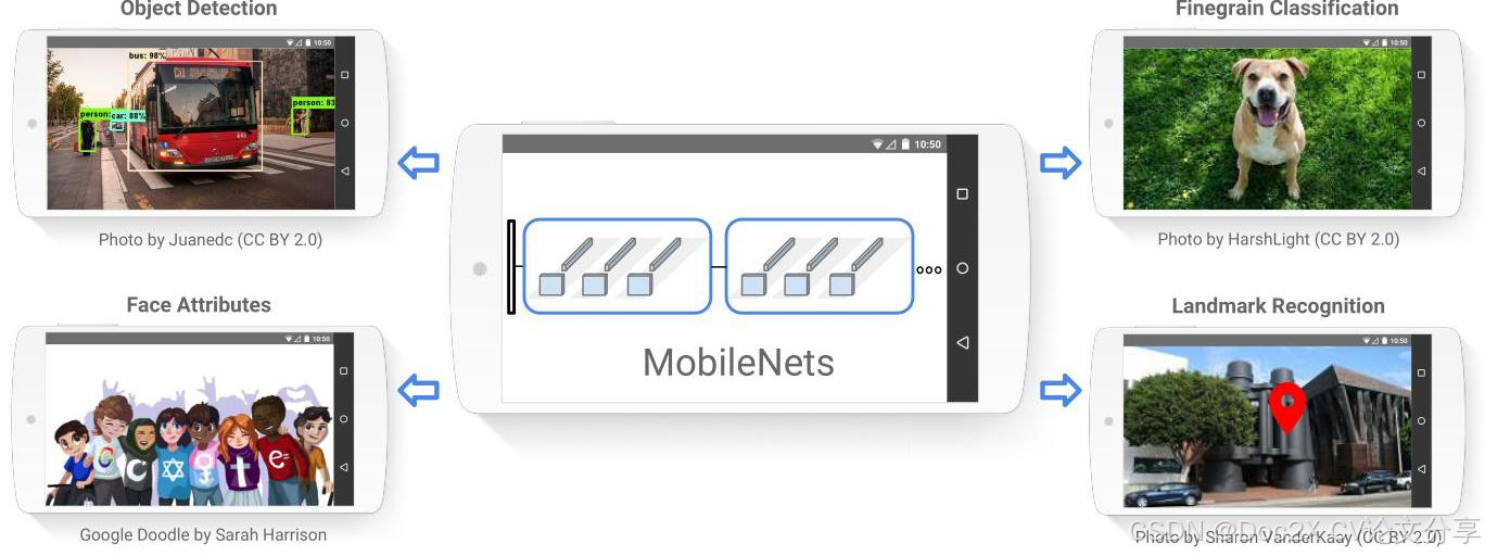
Figure 1. MobileNet models can be applied to various recognition tasks for efficient on device intelligence.

图1. MobileNet模型可以应用于各种识别任务，以实现高效的设备智能。

3. MobileNet Architecture

3. MobileNet架构

In this section we first describe the core layers that Mo-bileNet is built on which are depthwise separable filters. We then describe the MobileNet network structure and conclude with descriptions of the two model shrinking hyper-parameters width multiplier and resolution multiplier.

在本节中，我们首先描述MobileNet所基于的核心层，即深度可分离卷积。然后我们描述MobileNet的网络结构，并以对两个模型缩小超参数宽度乘数和分辨率乘数的描述结束。

3.1. Depthwise Separable Convolution

3.1. 深度可分离卷积

The MobileNet model is based on depthwise separable convolutions which is a form of factorized convolutions which factorize a standard convolution into a depthwise convolution and a $1\times 1$ convolution called a pointwise convolution. For MobileNets the depthwise convolution applies a single filter to each input channel. The pointwise convolution then applies a $1\times 1$ convolution to combine the outputs the depthwise convolution. A standard convolution both filters and combines inputs into a new set of outputs in one step. The depthwise separable convolution splits this into two layers, a separate layer for filtering and a separate layer for combining. This factorization has the effect of drastically reducing computation and model size. Figure 2 shows how a standard convolution 2(a) is factorized into a depthwise convolution 2(b) and a $1\times 1$ pointwise convolution 2©.

MobileNet模型基于深度可分离卷积，这是一种将标准卷积因式分解为深度卷积和称为点卷积的 $1\times 1$ 卷积的因式分解卷积形式。对于MobileNet，深度卷积对每个输入通道应用一个单独的滤波器。然后，点卷积对深度卷积的输出应用 $1\times 1$ 卷积以进行组合。标准卷积在一步中同时过滤和组合输入，生成一组新的输出。深度可分离卷积将其分为两个层，一个用于过滤，另一个用于组合。这种因式分解显著减少了计算量和模型大小。图2显示了标准卷积2(a)是如何因式分解为深度卷积2(b)和 $1\times 1$ 点卷积2©的。

A standard convolutional layer takes as input a $D_F\times$

标准卷积层的输入为 $D_F\times$

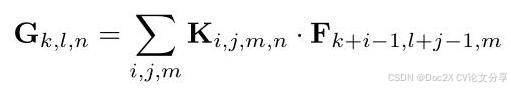
$D_F\times M$ feature map $\mathbf{F}$ and produces a $D_F\times D_F\times N$ feature map $\mathbf{G}$ where $D_F$ is the spatial width and height of a square input feature ${\mathrm{map}}^1,M$ is the number of input channels (input depth), $D_G$ is the spatial width and height of a square output feature map and $N$ is the number of output channel (output depth).

$D_F\times M$ 特征图 $\mathbf{F}$ 生成一个 $D_F\times D_F\times N$ 特征图 $\mathbf{G}$，其中 $D_F$ 是输入特征的空间宽度和高度， ${\mathrm{map}}^1,M$ 是输入通道的数量（输入深度）， $D_G$ 是输出特征图的空间宽度和高度， $N$ 是输出通道的数量（输出深度）。

The standard convolutional layer is parameterized by convolution kernel $\mathbf{K}$ of size $D_K\times D_K\times M\times N$ where $D_K$ is the spatial dimension of the kernel assumed to be square and $M$ is number of input channels and $N$ is the number of output channels as defined previously.

标准卷积层由卷积核 $\mathbf{K}$ 参数化，大小为 $D_K\times D_K\times M\times N$，其中 $D_K$ 是假设为正方形的卷积核的空间维度， $M$ 是输入通道的数量， $N$ 是之前定义的输出通道的数量。

The output feature map for standard convolution assuming stride one and padding is computed as:

假设步幅为1且有填充的标准卷积的输出特征图计算如下：

Standard convolutions have the computational cost of:

标准卷积的计算成本为：

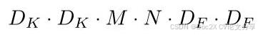
where the computational cost depends multiplicatively on the number of input channels $M$ ,the number of output channels $N$ the kernel size $D_k\times D_k$ and the feature map size $D_F\times D_F$ . MobileNet models address each of these terms and their interactions. First it uses depthwise separable convolutions to break the interaction between the number of output channels and the size of the kernel.

其中计算成本与输入通道的数量 $M$、输出通道的数量 $N$、卷积核大小 $D_k\times D_k$ 和特征图大小 $D_F\times D_F$ 成乘法关系。MobileNet模型解决了这些项及其相互作用。首先，它使用深度可分离卷积来打破输出通道数量与卷积核大小之间的相互作用。

The standard convolution operation has the effect of filtering features based on the convolutional kernels and combining features in order to produce a new representation. The filtering and combination steps can be split into two steps via the use of factorized convolutions called depthwise separable convolutions for substantial reduction in computational cost.

标准卷积操作的效果是基于卷积核对特征进行过滤，并结合特征以生成新的表示。通过使用称为深度可分离卷积的分解卷积，可以将过滤和组合步骤分为两个步骤，从而显著降低计算成本。

---

${}^1$ We assume that the output feature map has the same spatial dimensions as the input and both feature maps are square. Our model shrinking results generalize to feature maps with arbitrary sizes and aspect ratios.

${}^1$ 我们假设输出特征图与输入具有相同的空间维度，并且两个特征图都是正方形。我们的模型缩小结果可以推广到具有任意大小和纵横比的特征图。

---

Depthwise separable convolution are made up of two layers: depthwise convolutions and pointwise convolutions. We use depthwise convolutions to apply a single filter per each input channel (input depth). Pointwise convolution, a simple $1\times 1$ convolution,is then used to create a linear combination of the output of the depthwise layer. MobileNets use both batchnorm and ReLU nonlinearities for both layers.

深度可分离卷积由两层组成：深度卷积和逐点卷积。我们使用深度卷积为每个输入通道（输入深度）应用一个滤波器。然后使用逐点卷积，这是一种简单的 $1\times 1$ 卷积，来创建深度层输出的线性组合。MobileNets 在这两层中都使用批归一化和 ReLU 非线性激活函数。

Depthwise convolution with one filter per input channel (input depth) can be written as:

每个输入通道（输入深度）使用一个滤波器的深度卷积可以写成：

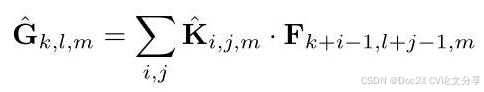
where $\hat{\mathbf{K}}$ is the depthwise convolutional kernel of size $D_K\times D_K\times M$ where the $m_{th}$ filter in $\hat{\mathbf{K}}$ is applied to the $m_{th}$ channel in $\mathbf{F}$ to produce the $m_{th}$ channel of the filtered output feature map $\hat{\mathbf{G}}$ .

其中 $\hat{\mathbf{K}}$ 是大小为 $D_K\times D_K\times M$ 的深度卷积核，$\hat{\mathbf{K}}$ 中的 $m_{th}$ 滤波器应用于 $\mathbf{F}$ 中的 $m_{th}$ 通道，以生成过滤后的输出特征图 $\hat{\mathbf{G}}$ 的 $m_{th}$ 通道。

Depthwise convolution has a computational cost of:

深度卷积的计算成本为：

Depthwise convolution is extremely efficient relative to standard convolution. However it only filters input channels, it does not combine them to create new features. So an additional layer that computes a linear combination of the output of depthwise convolution via $1\times 1$ convolution is needed in order to generate these new features.

相对于标准卷积，深度卷积的效率极高。然而，它仅对输入通道进行过滤，并不将它们组合以创建新特征。因此，需要一个额外的层，通过 $1\times 1$ 卷积计算深度卷积输出的线性组合，以生成这些新特征。

The combination of depthwise convolution and $1\times 1$ (pointwise) convolution is called depthwise separable convolution which was originally introduced in [26].

深度卷积和 $1\times 1$（逐点）卷积的组合称为深度可分离卷积，最初在 [26] 中提出。

Depthwise separable convolutions cost:

深度可分离卷积的成本为：

which is the sum of the depthwise and $1\times 1$ pointwise convolutions.

这是深度卷积和 $1\times 1$ 逐点卷积的总和。

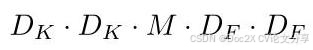
By expressing convolution as a two step process of filtering and combining we get a reduction in computation of:

通过将卷积表示为过滤和组合的两步过程，我们在计算上得到了减少：

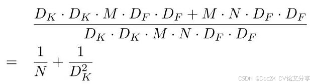
MobileNet uses $3\times 3$ depthwise separable convolutions which uses between 8 to 9 times less computation than standard convolutions at only a small reduction in accuracy as seen in Section 4.

MobileNet 使用 $3\times 3$ 深度可分离卷积，其计算量比标准卷积少 8 到 9 倍，同时准确度仅略有下降，如第 4 节所示。

Additional factorization in spatial dimension such as in $\left[16,31\right]$ does not save much additional computation as very little computation is spent in depthwise convolutions.

在空间维度上的额外因式分解，例如在 $\left[16,31\right]$ 中，并没有节省太多额外的计算，因为在深度卷积中花费的计算非常少。

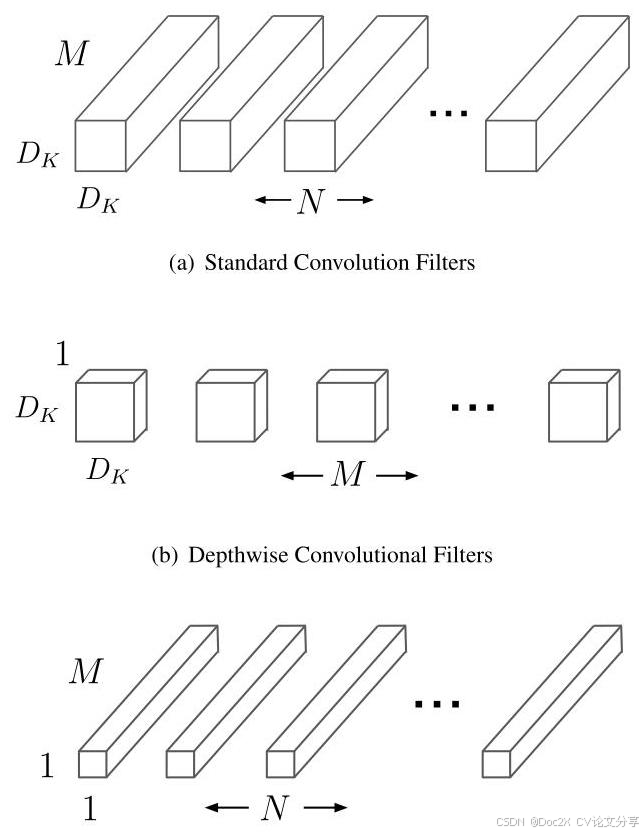
© $1\times 1$ Convolutional Filters called Pointwise Convolution in the context of Depthwise Separable Convolution

© $1\times 1$ 在深度可分离卷积的背景下称为逐点卷积的卷积滤波器

Figure 2. The standard convolutional filters in (a) are replaced by two layers: depthwise convolution in (b) and pointwise convolution in © to build a depthwise separable filter.

图2. (a) 中的标准卷积滤波器被两个层替代： (b) 中的深度卷积和 © 中的逐点卷积，以构建深度可分离滤波器。

3.2. Network Structure and Training

3.2. 网络结构与训练

The MobileNet structure is built on depthwise separable convolutions as mentioned in the previous section except for the first layer which is a full convolution. By defining the network in such simple terms we are able to easily explore network topologies to find a good network. The MobileNet architecture is defined in Table 1. All layers are followed by a batchnorm [13] and ReLU nonlinearity with the exception of the final fully connected layer which has no nonlinearity and feeds into a softmax layer for classification. Figure 3 contrasts a layer with regular convolutions, batchnorm and ReLU nonlinearity to the factorized layer with depthwise convolution, $1\times 1$ pointwise convolution as well as batch-norm and ReLU after each convolutional layer. Down sampling is handled with strided convolution in the depthwise convolutions as well as in the first layer. A final average pooling reduces the spatial resolution to 1 before the fully connected layer. Counting depthwise and pointwise convolutions as separate layers, MobileNet has 28 layers.

MobileNet 结构建立在深度可分离卷积的基础上，如前一节所述，第一层是全卷积。通过以如此简单的方式定义网络，我们能够轻松探索网络拓扑，以找到一个良好的网络。MobileNet 架构在表1中定义。所有层后面都跟有批归一化 [13] 和 ReLU 非线性，唯一的例外是最后的全连接层，该层没有非线性，并且输入到 softmax 层进行分类。图3 对比了具有常规卷积、批归一化和 ReLU 非线性的层与具有深度卷积、$1\times 1$ 逐点卷积以及在每个卷积层后进行的批归一化和 ReLU 的分解层。下采样通过深度卷积和第一层中的步幅卷积来处理。最终的平均池化将空间分辨率降低到 1，然后进入全连接层。将深度卷积和逐点卷积视为单独的层，MobileNet 共有 28 层。

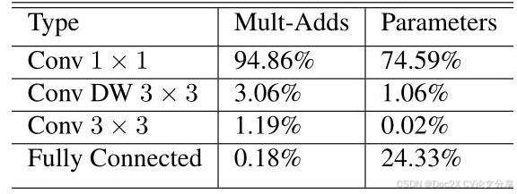
It is not enough to simply define networks in terms of a small number of Mult-Adds. It is also important to make sure these operations can be efficiently implementable. For instance unstructured sparse matrix operations are not typically faster than dense matrix operations until a very high level of sparsity. Our model structure puts nearly all of the computation into dense $1\times 1$ convolutions. This can be implemented with highly optimized general matrix multiply (GEMM) functions. Often convolutions are implemented by a GEMM but require an initial reordering in memory called im2col in order to map it to a GEMM. For instance, this approach is used in the popular Caffe package [15]. $1\times 1$ convolutions do not require this reordering in memory and can be implemented directly with GEMM which is one of the most optimized numerical linear algebra algorithms. MobileNet spends $95\%$ of it’s computation time in $1\times 1$ convolutions which also has $75\%$ of the parameters as can be seen in Table 2. Nearly all of the additional parameters are in the fully connected layer.

仅仅通过少量的 Mult-Adds 定义网络是不够的。确保这些操作可以高效实现同样重要。例如，非结构稀疏矩阵操作通常在稀疏度非常高之前并不比密集矩阵操作更快。我们的模型结构几乎将所有计算都放在密集 $1\times 1$ 卷积中。这可以通过高度优化的通用矩阵乘法（GEMM）函数实现。通常，卷积是通过 GEMM 实现的，但需要在内存中进行初始重排，称为 im2col，以便将其映射到 GEMM。例如，这种方法在流行的 Caffe 包中被使用 [15]。 $1\times 1$ 卷积不需要在内存中进行这种重排，可以直接通过 GEMM 实现，而 GEMM 是最优化的数值线性代数算法之一。MobileNet 在 $1\times 1$ 卷积中花费了 $95\%$ 的计算时间，这也具有 $75\%$ 的参数，如表 2 所示。几乎所有额外的参数都在全连接层中。

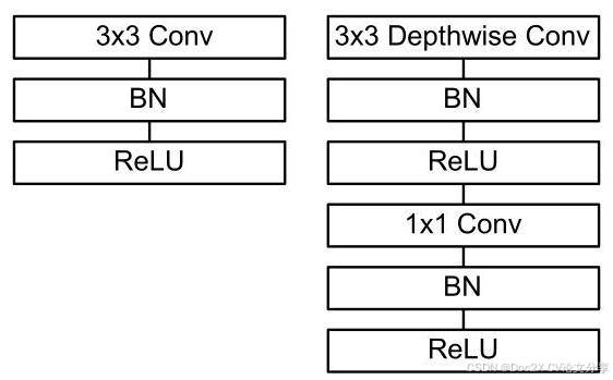
Figure 3. Left: Standard convolutional layer with batchnorm and ReLU. Right: Depthwise Separable convolutions with Depthwise and Pointwise layers followed by batchnorm and ReLU.

图 3. 左：标准卷积层，带有批归一化和 ReLU。右：深度可分离卷积，包含深度卷积和逐点卷积层，后接批归一化和 ReLU。

MobileNet models were trained in TensorFlow [1] using RMSprop [33] with asynchronous gradient descent similar to Inception V3 [31]. However, contrary to training large models we use less regularization and data augmentation techniques because small models have less trouble with overfitting. When training MobileNets we do not use side heads or label smoothing and additionally reduce the amount image of distortions by limiting the size of small crops that are used in large Inception training [31]. Additionally, we found that it was important to put very little or no weight decay (12 regularization) on the depthwise filters since their are so few parameters in them. For the ImageNet benchmarks in the next section all models were trained with same training parameters regardless of the size of the model.

MobileNet 模型是在 TensorFlow [1] 中使用 RMSprop [33] 进行训练的，采用与 Inception V3 [31] 类似的异步梯度下降。然而，与训练大型模型相反，我们使用更少的正则化和数据增强技术，因为小型模型在过拟合方面遇到的困难较少。在训练 MobileNets 时，我们不使用侧头或标签平滑，并且通过限制用于大型 Inception 训练 [31] 的小裁剪的大小来减少图像失真的数量。此外，我们发现对深度可分离卷积的滤波器施加很少或不施加权重衰减（12 正则化）是很重要的，因为它们的参数非常少。在下一节的 ImageNet 基准测试中，所有模型都使用相同的训练参数进行训练，无论模型的大小如何。

3.3. Width Multiplier: Thinner Models

3.3. 宽度乘数：更细的模型

Although the base MobileNet architecture is already small and low latency, many times a specific use case or application may require the model to be smaller and faster. In order to construct these smaller and less computationally expensive models we introduce a very simple parameter $\alpha$ called width multiplier. The role of the width multiplier $\alpha$ is to thin a network uniformly at each layer. For a given layer and width multiplier $\alpha$ ,the number of input channels $M$ becomes $\alpha M$ and the number of output channels $N$ becomes $\alpha N$ .

尽管基础的 MobileNet 架构已经很小且延迟低，但许多特定的用例或应用可能要求模型更小且更快。为了构建这些更小且计算成本更低的模型，我们引入了一个非常简单的参数 $\alpha$，称为宽度乘数。宽度乘数 $\alpha$ 的作用是在每一层均匀地缩小网络。对于给定的层和宽度乘数 $\alpha$，输入通道的数量 $M$ 变为 $\alpha M$，输出通道的数量 $N$ 变为 $\alpha N$。

Table 1. MobileNet Body Architecture

表 1. MobileNet 主体架构

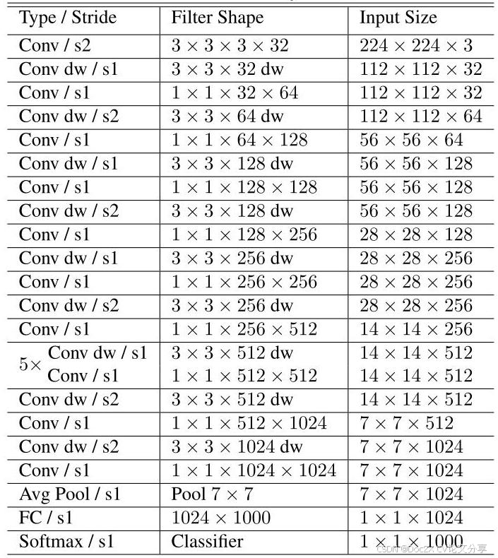
Table 2. Resource Per Layer Type

表 2. 每层类型的资源

The computational cost of a depthwise separable convolution with width multiplier $\alpha$ is:

带有宽度乘数 $\alpha$ 的深度可分离卷积的计算成本为：

where $\alpha \in (0,1]$ with typical settings of1,0.75,0.5and 0.25. $\alpha =1$ is the baseline MobileNet and $\alpha <1$ are reduced MobileNets. Width multiplier has the effect of reducing computational cost and the number of parameters quadratically by roughly ${\alpha }^2$ . Width multiplier can be applied to any model structure to define a new smaller model with a reasonable accuracy, latency and size trade off. It is used to define a new reduced structure that needs to be trained from scratch.

在 $\alpha \in (0,1]$ 的典型设置下为 1, 0.75, 0.5 和 0.25。$\alpha =1$ 是基线 MobileNet，而 $\alpha <1$ 是减少后的 MobileNet。宽度乘数的效果是以大约 ${\alpha }^2$ 的方式二次减少计算成本和参数数量。宽度乘数可以应用于任何模型结构，以定义一个新的较小模型，具有合理的准确性、延迟和大小权衡。它用于定义一个需要从头开始训练的新减少结构。

3.4. Resolution Multiplier: Reduced Representa- tion

3.4. 分辨率乘数：减少表示

The second hyper-parameter to reduce the computational cost of a neural network is a resolution multiplier $\rho$ . We ap-

减少神经网络计算成本的第二个超参数是分辨率乘数 $\rho$。我们应用-

—— 更多内容请到Doc2X翻译查看——
—— For more content, please visit Doc2X for translations ——