VS2019C++调用Python方法绘制频率直方图和正态分布

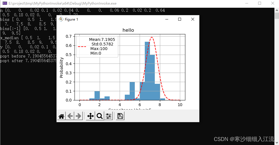
目的：通过VS C++代码中调用python文件执行正太曲线绘制；

1.首先先安装python环境：

安装方法百度下就可以了，我这里是通过anaconda安装的python

C++如何调用python可以参考官方链接：1. Embedding Python in Another Application — Python 3.5.9 documentation

2.参考链接：

C++中调用python(VS2017) - 知乎

C++调用python文件（包含第三方库） - 知乎

C++调python(执行py文件) - 知乎

3.建立vs工程：

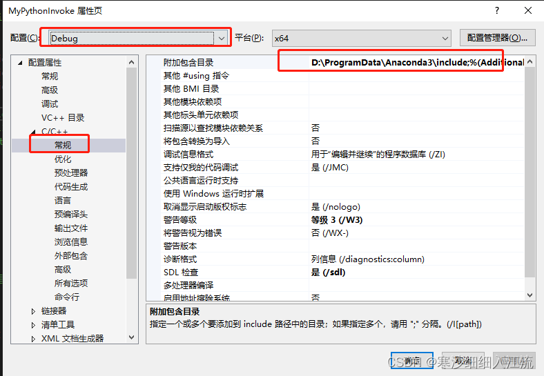
配置项目中的python头文件

​

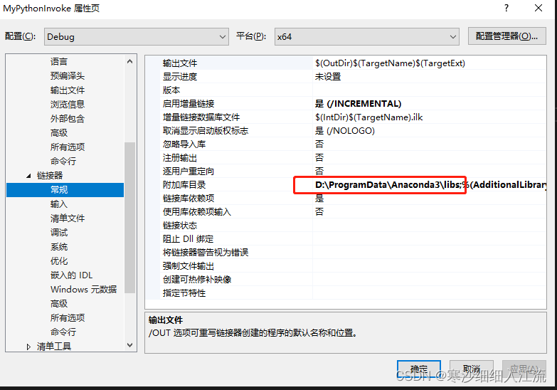
配置项目中的python库目录和库名称

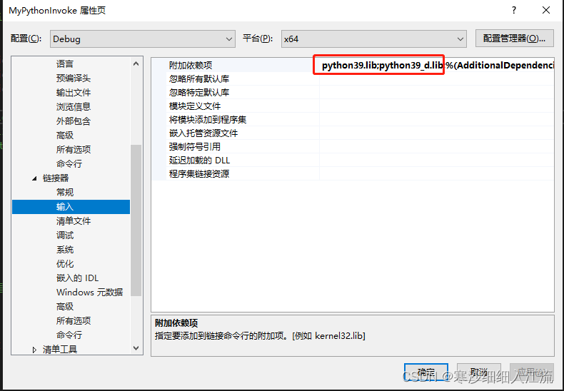
 python39_d.lib是python39.lib的拷贝文件；都是从python中拷贝过来的

 4.项目源代码： 

//hkk.py
import numpy as np
import matplotlib.pyplot as plt
from scipy.optimize import curve_fit
import scipy.stats as stats
import math

def func1():
     print("Hello test!")
     return 1;
 

def gaussian(x, *param):
    return (1/(math.sqrt(2*math.pi)*param[1])) * np.exp(-np.power(x - param[0], 2.) / (2 * np.power(param[1], 2.)))


def plot_histogram_():

    x_max = 100
    x_min = 0
    
    # Fixing random state for reproducibility
    np.random.seed(19680801)
    # Fixing bin edges
    # HIST_BINS = np.linspace(0, 6, 100)

    # histogram our data with numpy
    # data = np.random.randn(10000)
    # data =  [7.2654, 2.03277, 6.76334, 7.00338, 6.14913, 1.9775, 2.39404, 6.12634, 7.35134, 6.7655, 1.36597, 5.2713, 7.21664, 7.37915, 6.6744, 1.74003, 7.72338, 7.60908, 6.72006, 5.14625, 5.00783, 1.73177, 1.76857, 6.69649, 1.77922, 2.2017, 1.83062, 1.95377, 7.00296, 7.31169, 5.9294, 7.24258, 2.24411, 2.2155, 7.66734, 2.82456, 1.67877, 7.76167, 6.93592, 7.20611, 2.38782, 1.88987, 7.35963, 6.91655, 6.20476, 5.10936, 1.71087, 6.93359, 5.0883, 7.46636, 7.15289, 1.83525, 4.94843, 1.96966, 7.62138, 6.34175, 2.38174, 6.74939, 2.11311, 6.83046, 2.0208, 7.42635, 1.94872, 1.38055, 7.13142, 5.18174, 2.38545, 1.74536, 6.41837, 7.131, 7.52165, 7.42459, 2.30149, 2.24742, 6.9972, 6.44297, 7.33294, 7.04717, 4.85079, 4.93295, 6.01496, 6.26122, 7.4935, 6.85164, 7.2565, 1.9032, 2.069, 1.93437, 4.99958, 6.26219, 5.16512, 6.97014, 7.05683, 7.19481, 2.06861, 6.70399, 6.58828, 6.44693, 2.32096, 4.97223]
    # data =  [7.88894, 1.3467, 6.65849, 7.7804, 1.83257, 6.97018, 2.34037, 7.44047, 6.80127, 6.56404, 7.16245, 7.24855, 2.14255, 6.43262, 6.94469, 6.39296, 1.82529, 6.81622, 7.48624, 6.36761, 7.70207, 7.39336, 7.14797, 5.02435, 7.13796, 6.79353, 6.60382, 4.7858, 6.97086, 6.10893, 6.97904, 7.54451, 7.38055, 4.99217, 8.00206, 7.10882, 6.42302, 6.79158, 7.33844, 6.9109, 5.91913, 7.5789, 7.02633, 1.85777, 5.08794, 6.72307, 4.90149, 6.55256, 1.9027, 7.08329, 7.04607, 7.21862, 7.16722, 6.69888, 6.98244, 4.95856, 7.19087, 2.23764, 4.77028, 7.44058, 7.11784, 7.20815, 6.27515, 6.76372, 7.31652, 6.69494, 6.9524, 7.45431, 6.73223, 5.00514, 7.50749, 7.00254, 7.16493, 7.201, 1.88949, 6.71638, 6.64678, 7.08118, 6.50866, 1.59007, 6.50723, 6.99344, 6.76795, 6.76383, 7.82885, 7.20419, 7.39873, 7.58324, 6.75968, 6.90544, 7.03643, 7.23384, 6.58306, 6.79961, 7.15919, 4.88223, 1.96755, 6.68077, 5.88991, 7.47127]
    # data =  [6.65763, 7.36857, 7.29674, 7.11361, 6.64974, 7.02747, 4.92898, 6.78555, 6.91713, 6.91148, 7.50278, 7.01796, 7.48314, 7.10297, 5.62539, 6.80757, 7.05147, 6.99843, 7.0223, 6.73806, 6.667, 6.74416, 7.31848, 6.86536, 5.06178, 1.53764, 4.99516, 6.70996, 2.32433, 5.02935, 7.47327, 7.18461, 7.13062, 6.66355, 1.45209, 2.24945, 5.03329, 6.79626, 1.82663, 7.04732, 2.11641, 6.42652, 7.83337, 7.33993, 7.28045, 7.07749, 7.57386, 6.68628, 5.06846, 7.60152, 6.45608, 5.077, 7.33552, 6.68061, 4.993, 7.22773, 7.06728, 6.74474, 7.43859, 6.91553, 6.66261, 6.91153, 7.64873, 6.86744, 7.6727, 6.45961, 6.56108, 7.30055, 7.19704, 4.96982, 6.73773, 7.33749, 1.69832, 7.12851, 6.84009, 6.97748, 7.14796, 6.59139, 7.09696, 7.57651, 7.11043, 1.86096, 6.55495, 7.15291, 6.72031, 7.70708, 5.01495, 5.18389, 7.13966, 6.9135, 6.83973, 5.09173, 7.41922, 2.17958, 4.84244, 6.43243, 7.32303, 6.99624, 7.32565, 7.41254]
    # data = [7.32903, 7.17183, 2.02648, 2.11705, 5.07626, 7.36888, 5.11512, 7.08272, 2.14369, 1.94483, 1.94185, 7.15878, 5.08155, 6.29721, 7.25878, 4.97784, 2.11403, 1.69539, 6.52666, 6.45935, 5.03949, 7.39002, 4.87624, 6.90869, 2.56274, 6.81552, 5.03895, 2.19283, 7.00192, 7.35649, 5.05341, 6.65124, 2.1801, 2.21088, 7.43335, 6.94916, 4.82815, 6.83361, 4.97302, 6.90525, 7.59127, 7.55913, 1.65296, 7.4794, 4.86088, 2.31297, 7.12617, 6.72091, 2.18809, 1.76027, 6.97936, 2.39315, 6.86662, 1.79574, 7.36421, 5.00541, 7.30526, 6.71656, 6.99752, 7.39532, 7.11338, 6.95899, 6.88974, 2.20865, 7.11952, 7.14588, 4.91891, 1.9052, 7.19167, 6.47373, 2.17401, 4.99841, 2.19322, 6.82869, 7.27367, 2.21578, 2.14636, 1.93288, 4.77814, 7.3725, 1.83752, 6.84817, 5.0789, 1.87859, 2.61552, 5.11605, 6.38427, 6.93952, 7.27008, 4.98622, 2.76918, 2.40666, 1.84567, 7.11203, 5.13611, 2.00969, 2.02367, 7.01861, 6.9348, 2.46768]
    # data = data<10
    #good
    data = [6.33965, 2.55212, 6.51941, 7.31259, 6.951, 7.28915, 5.81703, 6.76177, 7.17638, 7.11856, 1.87, 7.16429, 6.75712, 7.41274, 2.74875, 1.78699, 7.49564, 2.04678, 7.36245, 6.91319, 7.68733, 4.95401, 6.70903, 6.49051, 6.4956, 1.74239, 6.67, 7.71036, 5.10516, 7.43492, 6.89023, 7.10158, 6.93651, 7.4033, 4.97209, 7.90861, 7.12402, 7.03959, 5.03158, 7.26962, 7.72467, 6.4842, 6.98065, 7.29316, 7.79847, 5.09871, 7.30079, 6.87452, 4.95666, 5.09111, 7.6573, 6.55885, 6.01661, 6.68607, 7.01758, 6.16136, 7.62088, 6.71225, 7.02648, 8.38502, 6.96683, 7.01398, 6.3056, 6.85018, 6.99697, 5.02085, 6.32971, 6.44303, 6.58673, 7.11636, 5.24504, 5.10223, 6.6765, 7.4667, 1.58002, 1.20294, 6.63096, 7.19103, 6.73679, 7.5736, 6.76727, 6.7336, 6.81139, 6.65099, 7.08824, 6.53932, 7.43189, 5.2183, 6.60102, 5.19081, 6.78822, 7.6721, 6.45881, 6.79589, 6.83989, 1.94275, 6.98623, 6.89738, 7.38303, 5.01202]

    mu =np.mean(data) 
    sigma =np.std(data)
    # calculate bin
    plt.figure(figsize=(5,3))
    n, bins, patches = plt.hist(data,range=(0,10),bins=20,density=1, alpha=0.75)     # 频率直方图 
    print("n", n,len(n))
    print("bins",bins,len(bins))
    half = bins[1]-bins[0]
    print("bins[:-1]",bins[:-1])
    x_median = bins[:-1] + half
    y = n 
    
    print("x_median",x_median,len(x_median))
    print("y", y,len(y))

    
    popt,pcov = curve_fit(gaussian,x_median,y,p0=[mu,sigma],maxfev=100000) 
    fit_mu = popt[0]
    fit_sigma = popt[1]
    print("popt before",popt[0],popt[1])
    y_fit = gaussian(x_median,*popt)
    print("popt after",popt[0],popt[1])
    curve_x = np.linspace(bins[0], bins[-1], 500)
    curve_y = stats.norm.pdf(curve_x, fit_mu, fit_sigma) #拟合一条最佳正态分布曲线y
    plt.grid(True)
    plt.plot(curve_x, curve_y, 'r--',label='Mean:{} \n  Std:{} \n Max:{} \n Min:{}'.format(round(fit_mu,4),round(fit_sigma,4),x_max,x_min))  #绘制y的曲线 
    plt.xlabel('Capacitance Value/pF')  #绘制x轴 
    plt.ylabel('Probability')  #绘制y轴 
    plt.title('hello  ')  
    plt.legend()
    plt.show()


# plot_histogram_()

// MyPythonInvoke.cpp : 此文件包含 "main" 函数。程序执行将在此处开始并结束。
#include <iostream>
#include <Python.h>
#include<string>
using namespace std;
int main()
{
	Py_Initialize();//使用python之前，要调用Py_Initialize();这个函数进行初始化

	PyRun_SimpleString("import sys");
	PyRun_SimpleString("sys.path.append('E:/project/tmp/MyPythonInvoke/MyPythonInvoke')");
	PyRun_SimpleString("sys.path.append('E:/project/tmp/MyPythonInvoke/MyPythonInvoke/DLLs')");
	PyRun_SimpleString("sys.path.append('E:/project/tmp/MyPythonInvoke/MyPythonInvoke/Lib')");

	//PyRun_SimpleString("import matplotlib.pyplot as plt"); /*调用python文件*/
	//PyRun_SimpleString("plt.plot([1,2,3,4], [12,3,23,231])"); /*调用python文件*/
	//PyRun_SimpleString("plt.show()"); /*调用python文件*/

	if (!Py_IsInitialized())
	{
		printf("初始化失败！");
		return 0;
	}

	PyObject* pModule = NULL;//声明变量
	PyObject* pFunc = NULL;// 声明变量
	pModule = PyImport_ImportModule("hkk");//这里是要调用的文件名
	if (pModule == NULL)
	{
		PyErr_Print();
		cout << "PyImport_ImportModule Fail!" << endl;
		return -1;
	}

#if 0
	pFunc = PyObject_GetAttrString(pModule, "func1");//这里是要调用的函数名
#else
	pFunc = PyObject_GetAttrString(pModule, "plot_histogram_");//这里是要调用的函数名
#endif
	PyObject* args2 = Py_BuildValue("i", 25);//给python函数参数赋值

	PyObject* pRet = PyObject_CallObject(pFunc, nullptr);//调用函数
	if(pRet == nullptr)
	{
		PyErr_Print();
		cout << "PyObject_CallObject Fail!" << endl;
	}
	int res = 0;
	PyArg_Parse(pRet, "i", &res);//转换返回类型
	cout << "res:" << res << endl;//输出结果

	Py_Finalize(); // 与初始化对应
	system("pause");
	return 0;

}

 5.运行结果

6.期间出现的问题

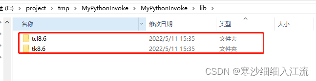
 出现了tcl 和tk版本不匹配的问题

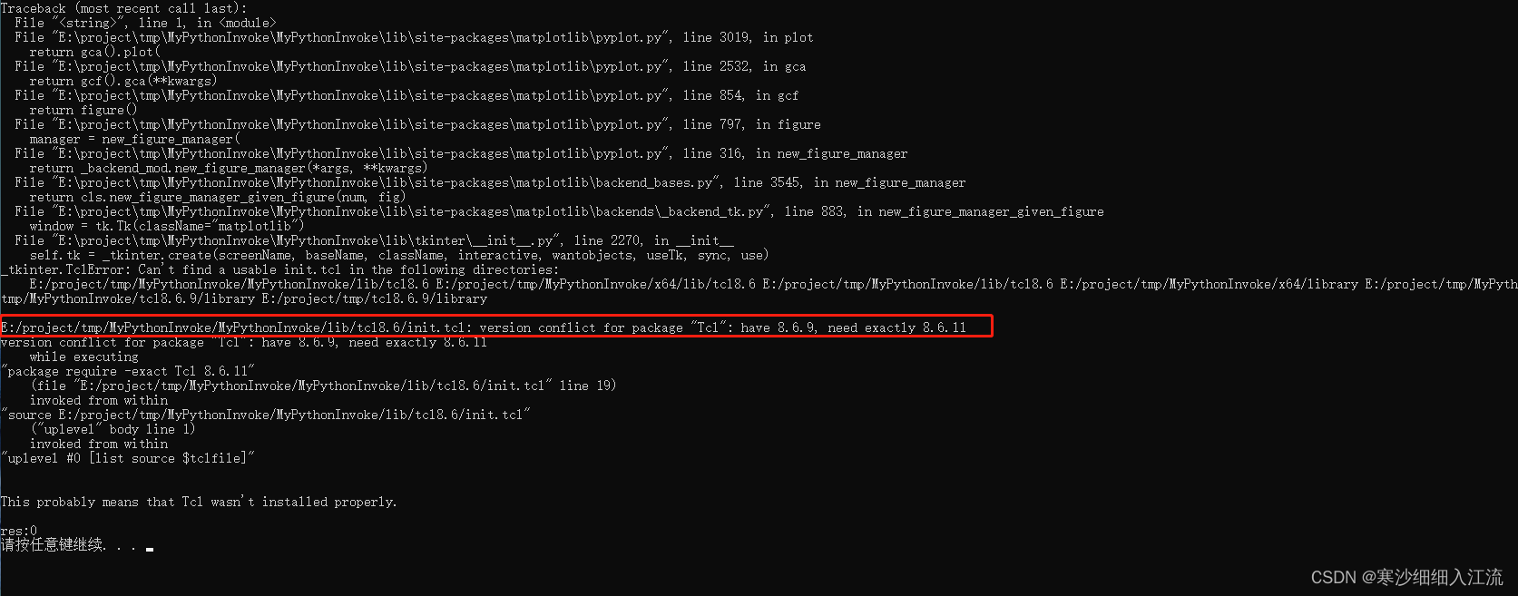
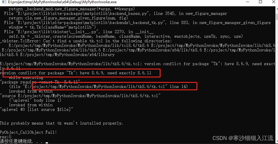
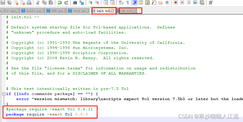
错误中标识tcl版本不匹配，错误中显示了寻找的目录位置，所以可以将python目录中的tcl8.6和tk8.6拷贝出来或者直接修改，则只需要将该文件修改为对应版本即可；

 

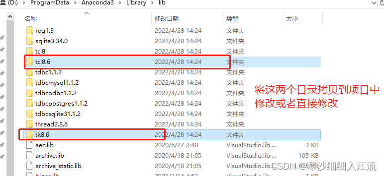
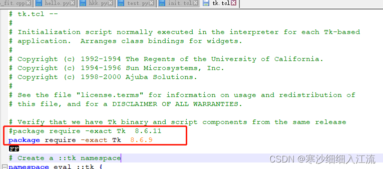
将文件init.tcl和文件tk.tcl 中8.6.11修改为8.6.9即可

 

7.源码下载

VS2019C++调用Python方法绘制频率直方图和正态分布-C++文档类资源-CSDN下载