Study notes for Anomaly Detection

Introduction

• Assume we have a data set including vast normal examples and only small anomalies. To detect these anomalies, we need to train a probabilistic model to determine whether a given example is anomaly or not.
  • p(x) refers to the probability that the example is normal. 
  • if flag this as an anomaly
  • if this is OK.
  • where  is a threshold that can be determined by maximizing the performance using cross validation.
  • Note that only normal examples (negative labels) are used to train the model.
  • Thus it can be regarded as an unsupervised learning algorithm.
• Applications
  • Fraud detection 
    • Some features can be used to describe a user's activity, such as length of online-time, login location, frequency, etc. 
    • Identify unusual users by checking anything that looks a bit weird
  • Manufacturing
    • Detect if a product looks good or not
  • Monitoring computers in data center
    • For a cluster of machines, we can model the use of each machine in terms of memory use, number of disk accesses/sec and CPU load, or defining our own complex features such as CPU load/network traffic
    • Detect whether an anomalous machine is able to fail or doing something abnormal. 
• The differences between anomaly detection and classification (or regression) are:
  • The data set only contains smaller number (typically 2-50) of examples as anomalies. Hence it may be not enough to "learn" a classifier or regressor, which require reasonably large number of positive and negative examples. 
  • There may be no suitable features (or existing any patterns) to describe those anomalies. For example, there are many "types" of anomalies. 

The Anomaly Detection Algorithm

• For a set of unlabeled training set: , assume if each example is n-dimensional, i.e. has n features. 
• Calculate parameters of all features  by
  
• Model p(x) as follows:
  
  • It is assumed that each feature is distributed according to a Gaussian distribution
  • There is no correlation between two features, i.e., all features are independent. 
  • Note that: the algorithm may still work if features are correlated. 
  • Besides, we can conduct dimension reduction (e.g. PCA) to solve this problem. 
• Compute p(x) and a test example x is anomaly if
• Performance measure: precision/recall, F-measure

Choose Features to Use

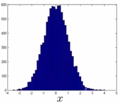
• Plot a histogram of data to check if it has a Gaussian distribution, although it may still works if data is non-Gaussian.
• Non-Gaussian data may look like this:
  
  We can use different transformation to make it look more Gaussian, e.g., log(x) transformation obtains:
  
  Hence, we can use log(x) rather than x as a feature. Other possible transformations include log(x+c) or x^0.5.
• Use error analysis, trying to interpret the performance of p(x) and come up with new features that can account for the errors. For example, the new feature CPU load/network traffic may be useful. 

Anomaly Detection with Multivariate Gaussian Distribution

• The new model based on multivariate Gaussian distribution is as follows:
  
  It can be rewritten as , or explicitly with m-dimensional  .
• The new parameters: 
  • is an n-dimensional mean vector, where n is the number of features. 
  •  is an [n x n] covariance matrix, including the correlaitons between different features. 
  •  is the absolute values of determinant of sigma. It can be computed in Matlab using det(sigma). 
• Calculate the parameters of features:
  

Multivariate Gaussian Distribution

• If features are not independent, but correlated with each with to some extent, then the simple anomaly detection may fail to work. 
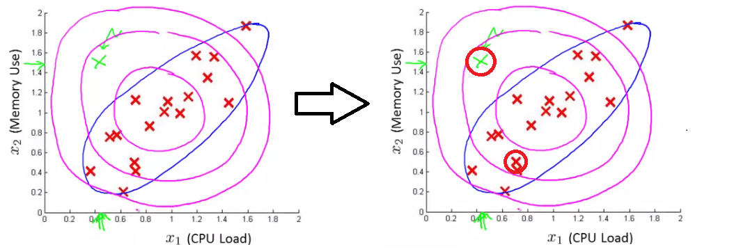
• For example, assume the data set is shown as follows:
  
  In this case, the test exmple may be regarded as "normal" by the previous anomaly detection (the checking areas are the circles). This is because the model makes probability prediction in concentric circles around the means of both. However, data in the blue ellipse are more likely to be normal and the test example is far from that. 
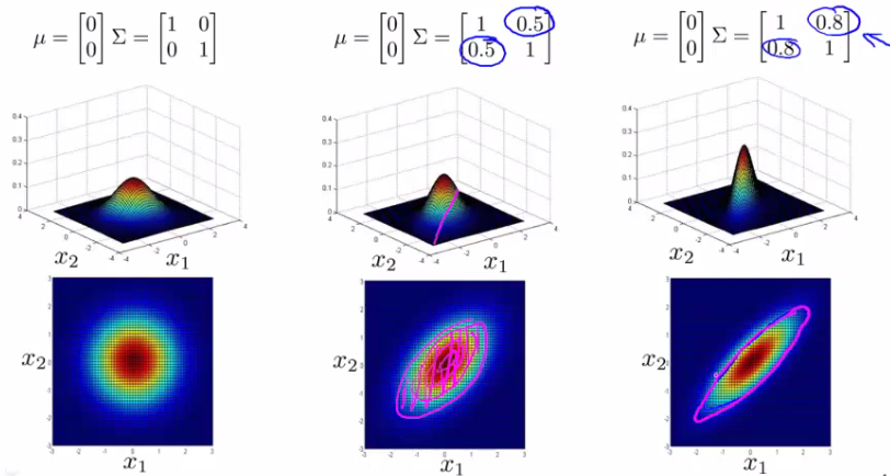
• The multivariate Gaussian distribution can be represented by:
  
  • It can be seen that the final example gives a very tall thin distribution, showing a strong positive correlation.
  • We can also make the off-diagonal values negative to show a negative correlation. 

Simple vs. Multivariante Gaussian

• Simple anomaly detection can be regarded as a special case of multivariate anomaly detection when features are independent, i.e., the covariance between different features is zero.
• Simple Gaussian model is more often used because 
  • It is cheaper to compute; 
  • It scales much better to very large feature vectors.
  • It works well with a small training set.
• Simple Gaussian model needs to manually create new features that capture the feature correlations. But it may be difficult in some cases.
• Multivariate model can automatically capture feature correlations via covariance matrix.
  • Hence it is more computationally expensive.
  • Needs for m>n, otherwise the covariance matrix is not invertible.
  • No redundant (or linearly dependent) features which also leads to matrix non-invertible. 

References

1. Anomaly Detection: http://www.holehouse.org/mlclass/15_Anomaly_Detection.html