Study notes for Expectation Maximum Algorithm

1. Introduction

• The EM algorithm is an efficient iterative procedure to compute the maximum likelihood (ML) estimate in the presence of missing or hidden data (variables). 
• It intends to estimate the model parameters such that the observed data are the most likely.

Convexity

• Let be a real function defined on an interval . is said to be convex on if,
  
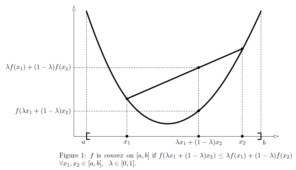
  is said to be strictly convex if the inequality is strict. Intuitively, this definition states that the function falls below (strictly convex) or is never above (convex) the straight line from points  to .
  
• is concave (strictly concave) if  is convex (strictly convex). 
• Theorem 1. If is twice differentiable on [a, b] and  on [a, b], then  is convex on [a, b].
  • If x takes vector values, f(x) is convex if the hessian matrix H is positive semi-definite (H>=0).
  • -ln(x) is strictly convex in (0, inf), and hence ln(x) is strictly concave in (0, inf).

Jensen's inequality

• The convexity is generalized to multivariate. 
• Let be a convex function defined on an interval. If and with,
  
  Note that holds true if and only if with probability 1, i.e., if X is a constant.
• Hence, for concave functions:
  
• Applying ln(x) and concavity, we can verify that,
  

2. The EM Algorithm

• Objective: maximize the log-likelihood of the data x, which is drawn from an unknown distribution, given the model parameterized by:
  
• The basic idea: 
  • Introduce a hidden variable such that its knowledge would simplify the maximization of 
  • Each iteration of the EM algorithm consists of two processes:
    • E-step: estimate the distribution of the hidden variable given the data and the current values of the parameters. 
    • M-step: modify the parameters in order to maximize the joint distribution of the data and the hidden variable.
• Convergence is assured since the algorithm is guaranteed to increase the likelihood at each iteration.
  My understanding: it is usually difficult to directly estimate or maximize the objective function, since there are so many parameters and the objective function may not be differentiable (hence it is not applicable of traditional differential methods). Instead, the EM algorithm introduces a hidden variable which makes it easy to estimate the parameter values. Specifically, it aims to maximize the joint distribution of the data and the hidden variable, which is corresponding to optimize and maximize the original objective function according to the convergence property of the EM algorithm. 
• The detailed derivation can be referred to Andrew's or Sean's tutorial. 

Example: EM for GMM (shortly), more can be found in the GMM study. 

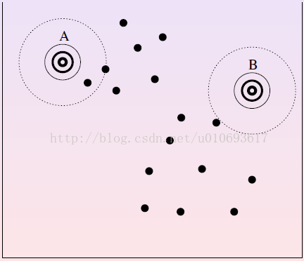
• Assume a hidden variable q, referring to for each point, which Gaussian generated it? (see left figure).
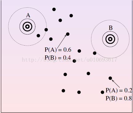
• E-step: for each point, estimate the probability that each Gaussian generated it.  (see middle figure).
• M-step: modify the parameters according to the hidden variable to maximize the likelihood of the data and the hidden variable.  (see right figure).
  Let us consider the following auxiliary function: . It aims to find the best parameters that maximize function A: 

References

1. Andrew Ng, The EM algorithm: http://cs229.stanford.edu/materials.html.  
2. Sean Borman, The Expectation Maximization Algorithm: a short tutorial. 
3. Samy Bengio, Statistical Machine Learning from Data Gaussian Mixture Models.