


前言
  从linux camera驱动, 到qcom平台 camera图像效果,再到opencv图像处理,终于进入本篇的机器学习的开始。
    前路漫漫,吾只愿风雨兼程。
简介
  本篇开始是学习机器学习的第一篇,本章主要是使用opencv,用c语言实现机器学习之一元线性回归、梯度下降法。
关于这部分的原理,可以参考:
        1、 http://studentdeng.github.io/blog/2014/07/28/machine-learning-tutorial/
        2、 https://www.coursera.org/learn/machine-learning/home/info
具体实现
大致流程
  首先创建了一个400x400的空白图片,在图片上,随机初始化了8个坐标点。这些坐标点的x和y坐标分别就是代替对应的数据集(比如x轴坐标代表
房屋面积,y坐标表示房屋价格)。
  接着利用公式: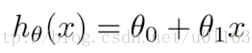
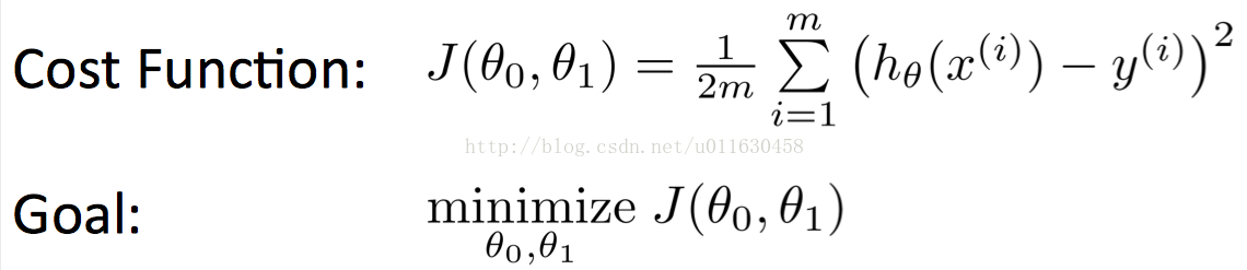
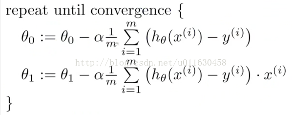
来连续迭代拟合出更加优秀的结果参数,并在之前的空白图片上不断更新出来。
实现代码
#include <opencv2/core/core.hpp>
#include <opencv2/highgui/highgui.hpp>
#include <math.h>
#include <string.h>
#include <opencv/cv.h>
#include <stdio.h>
#include "opencv2/photo/photo.hpp"
#include <unistd.h>

using namespace cv;

#define specimenNum  8
#define cir 5

char inputWindow[20] = "input";
Mat mat1;
int normalWidth=400, normalHeight=400;
int specimenAddr[specimenNum][2] = {{50, 150}, {150, 50}, {220, 220},{150, 150}, {300,300}, {70, 120}, {120, 70}, {160, 160}};
int funcNum[2] = {0, 0};
double k0=1, k1=10, j_tmp= 0;
bool step_flag = true;

/*******************************************
*********样本点初始化显示*******************
*******************************************/
void specimenInit(void){
	int i;

	mat1 = Mat(normalWidth, normalHeight, CV_8UC3, cv::Scalar(0, 0, 0));
	for(i=0; i<specimenNum; i++){
		Point center = Point(specimenAddr[i][0], specimenAddr[i][1]);
		circle(mat1, center, cir, Scalar(128,128,255), -1);
	}
	imshow(inputWindow, mat1);
}

/******************************************
*********画出当前学习曲线******************
*******************************************/
void drawmachinaline(void){
	double i, j, m, n;
	Mat matTmp;

	mat1.copyTo(matTmp);
	for(i=0; i< normalWidth; i++){
		n = (double)i;
		m = k0 + k1 * n;
		if(m <= normalHeight){
			Point center = Point((int)n, (int)m);
			circle(matTmp, center, 2, Scalar(255, 255, 255), -1);
		}
	}
	imshow(inputWindow, matTmp);
	waitKey(10);
}

/*******************************************
*********键值处理,按下q则退出**************
*******************************************/
void mykey(void){
	while(1){
		char c;
		c = waitKey(0);
		if(c == 'q'){
			break;
		}
	}
}

void computeCost(void){
	double j, tmp;
	int i;

	for(i=0; i<specimenNum; i++){
		tmp = tmp + (k0 + k1 * specimenAddr[i][0] - specimenAddr[i][1]) * \
		          (k0 + k1 * specimenAddr[i][0] - specimenAddr[i][1]);
	}
	j = tmp / specimenNum / 2;

	if(j < j_tmp){
		if(j_tmp - j  < 0.02){
			step_flag = false;
		}
		j_tmp = j;
	}else{
		if(j_tmp == 0){
			j_tmp = j;
		}else{
			step_flag = false;
		}
	}
	drawmachinaline();
	printf("j:%lf\n", j);
}

/*******************************************
*********计算最佳函数参数*******************
*******************************************/
void getfuncNum(void){
	double tmp0, tmp1, temp0, temp1;
	int i;
	bool flag = false;
	double aa = 100000;

	while(step_flag){
		temp0 = 0;
		temp1 = 0;

		for(i=0; i<specimenNum; i++){
			temp0 = temp0 + k0 + k1 * specimenAddr[i][0] - specimenAddr[i][1];
		}
		temp0 = temp0 / specimenNum / aa;
		tmp0 = k0 - temp0;

		for(i=0; i<specimenNum; i++){
			temp1 = temp1 + (k0 + k1 * specimenAddr[i][0] - specimenAddr[i][1]) * specimenAddr[i][0];
		}
		temp1 = temp1 / specimenNum / aa;
		tmp1 = k1 - temp1;
		if(k1 == tmp1){
			break;
		}
		k0 = tmp0;
		k1 = tmp1;
		computeCost();
		sleep(1);
	}
	printf("k0:%lf, k1:%lf\n", k0, k1);
}

int main(int argc, char *argv[]){

	specimenInit();
	getfuncNum();
	mykey();

	return 0;
}
代码讲解
1、首先是进行对应初始化操作。创建了一个空白图片,然后将代表数据集的样本点,画在图像对应位置。
void specimenInit(void){
	int i;

	mat1 = Mat(normalWidth, normalHeight, CV_8UC3, cv::Scalar(0, 0, 0));
	for(i=0; i<specimenNum; i++){
		Point center = Point(specimenAddr[i][0], specimenAddr[i][1]);
		circle(mat1, center, cir, Scalar(128,128,255), -1);
	}
	imshow(inputWindow, mat1);
}
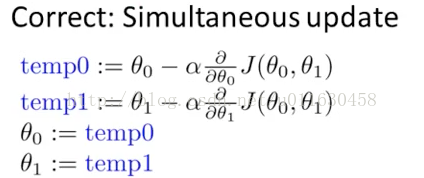
2、根据之前提到的公式,进行迭代更新参数。每次更新后的参数,放入k0和k1中,接着使用computeCost,计算代价函数值和将当前迭代的参数效果。
void getfuncNum(void){
	double tmp0, tmp1, temp0, temp1;
	int i;
	bool flag = false;
	double aa = 100000;

	while(step_flag){
		temp0 = 0;
		temp1 = 0;

		for(i=0; i<specimenNum; i++){
			temp0 = temp0 + k0 + k1 * specimenAddr[i][0] - specimenAddr[i][1];
		}
		temp0 = temp0 / specimenNum / aa;
		tmp0 = k0 - temp0;

		for(i=0; i<specimenNum; i++){
			temp1 = temp1 + (k0 + k1 * specimenAddr[i][0] - specimenAddr[i][1]) * specimenAddr[i][0];
		}
		temp1 = temp1 / specimenNum / aa;
		tmp1 = k1 - temp1;
		if(k1 == tmp1){
			break;
		}
		k0 = tmp0;
		k1 = tmp1;
		computeCost();
		sleep(1);
	}
	printf("k0:%lf, k1:%lf\n", k0, k1);
}
3、将当前迭代参数更新在图像上(k0,k1表示当前迭代参数),然后将图像显示出来。
void drawmachinaline(void){
	double i, j, m, n;
	Mat matTmp;

	mat1.copyTo(matTmp);
	for(i=0; i< normalWidth; i++){
		n = (double)i;
		m = k0 + k1 * n;
		if(m <= normalHeight){
			Point center = Point((int)n, (int)m);
			circle(matTmp, center, 2, Scalar(255, 255, 255), -1);
		}
	}
	imshow(inputWindow, matTmp);
	waitKey(10);
}
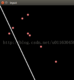
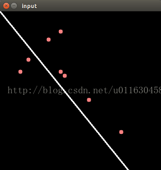
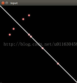
效果演示
迭代的效果演示如下: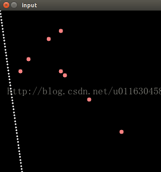


 1717
1717

 被折叠的 条评论
为什么被折叠?
被折叠的 条评论
为什么被折叠?
 到【灌水乐园】发言


