数字信号处理及python实现(三)

最新推荐文章于 2024-04-26 19:13:06 发布

飞华1993

最新推荐文章于 2024-04-26 19:13:06 发布

阅读量916

点赞数

分类专栏：科研文章标签： python 信号处理人工智能

本文链接：https://blog.csdn.net/u011740601/article/details/127873189

版权

科研专栏收录该内容

13 篇文章 4 订阅

订阅专栏

数字信号处理及python实现三

抽样引起的混叠
抽样的频域视图
样本重建信号
- 拟合正弦波
- 线性与多项式内插
理想低通滤波器

这是参考知乎的数字信号处理及matlab实现的python实现版本，参考连接

上一期:数字信号处理及python实现(二)

项目文件结构
在这里插入图片描述
test为测试文件，window为项目文件

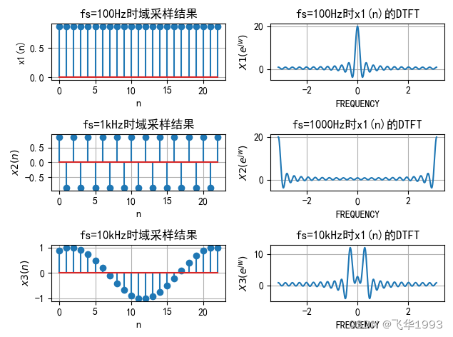
抽样引起的混叠

    def test_sample1(self):
        signal = Signal()
        f0 = 500
        n = np.array(list(range(0, 23)))
        fs1 = 100  # 采样频率为100Hz

        x1 = np.sin(2 * np.pi * f0 * n / fs1 + np.pi / 3)
        X1, W1 = signal.dtft(x1, 1000)  # 对x1进行DTFT变换
        fs2 = 1000  # 采样频率为1kHz
        x2 = np.sin(2 * np.pi * f0 * n / fs2 + np.pi / 3)
        X2, W2 = signal.dtft(x2, 1000)  # 对x2进行DTFT变换
        fs3 = 10000  # 采样频率为10kHz
        x3 = np.sin(2 * np.pi * f0 * n / fs3 + np.pi / 3)
        X3, W3 = signal.dtft(x3, 1000)  # 对x3进行DTFT变换

        plt.subplot(3, 2, 1);
        plt.stem(n, x1)  # 绘制fs = 100
        # Hz时域采样结果
        plt.title('fs=100Hz时域采样结果')
        plt.xlabel('n')
        plt.ylabel('x1(n)')
        plt.grid(visible=True)

        plt.subplot(3, 2, 2)
        plt.plot(W1, X1)
        plt.title('fs=100Hz时x1(n)的DTFT')
        plt.xlabel('FREQUENCY')
        plt.ylabel('$X1(e^{jw})$')
        plt.grid(visible=True)

        plt.subplot(3, 2, 3)
        plt.stem(n, x2)  # 绘制fs = 1
        # kHz时域采样结果
        plt.title('fs=1kHz时域采样结果')
        plt.xlabel('n')
        plt.ylabel('$x2(n)$')
        plt.grid(visible=True)

        plt.subplot(3, 2, 4)
        plt.plot(W2, X2)
        plt.title('fs=1000Hz时x1(n)的DTFT')
        plt.xlabel('FREQUENCY')
        plt.ylabel('$X2(e^{jw})$')
        plt.grid(visible=True)

        plt.subplot(3, 2, 5);
        plt.stem(n, x3)  # 绘制fs = 10
        # kHz时域采样结果
        plt.title('fs=10kHz时域采样结果')
        plt.xlabel('n')
        plt.ylabel('$x3(n)$')
        plt.grid(visible=True)

        plt.subplot(3, 2, 6)
        plt.plot(W3, X3)
        plt.title('fs=10kHz时x1(n)的DTFT')
        plt.xlabel('FREQUENCY')
        plt.ylabel('$X3(e^{jw})$')
        plt.grid(visible=True)

        plt.tight_layout()
        plt.savefig('data/images/sample1.png')

在这里插入图片描述

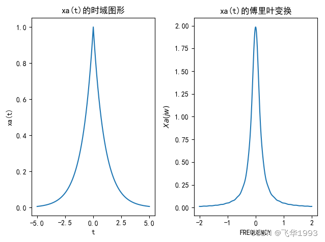
抽样的频域视图

    def test_sample_fourier(self):
        dt = 0.00001  # 给出一个无限小的间隔
        t = np.arange(-0.005, 0.005 + dt, dt)  # 给出t的取值范围

        xa = np.exp(-1000 * abs(t))  # xa的时域表达式
        Wmax = 2 * np.pi * 2000  # 给出频率的最大值
        K = 600
        k = np.array(list(range(0, K + 1)))
        W = k * Wmax / K  # W的范围
        Xa = np.array(np.matrix(xa) * np.exp(np.complex(0, -1) * np.matrix(t).T * np.matrix(W)) * dt)
        Xa = np.real(Xa)  # 连续时间傅里叶变换
        len_W = len(W)
        W.resize(1, len_W)

        W = np.concatenate([-np.fliplr(W)[0], W[0][1:]], axis=0)  # 给出频率的范围
        Xa = np.concatenate([np.fliplr(Xa)[0], Xa[0][1:]], axis=0)  # 给出Xa的范围

        plt.subplot(1, 2, 1)
        plt.plot(t * 1000, xa)  # 绘出xa(t)的时域图形
        plt.title('xa(t)的时域图形')
        plt.xlabel('t')
        plt.ylabel('xa(t)')

        plt.subplot(1, 2, 2)
        plt.plot(W / (2 * np.pi * 1000), Xa * 1000)  # 绘出xa(t)的傅里叶变换的频谱
        plt.title('xa(t)的傅里叶变换')
        plt.xlabel('FREQUENCY')
        plt.ylabel('$Xa(jw)$')

        plt.tight_layout()
        plt.savefig('data/images/sample_fourier.png')

在这里插入图片描述
e.g. $x_a(t)=e^{-1000|t|}$ ，绘制其傅里叶变换 $X_a(j\Omega)$

    def test_sample_fourier(self):
        dt = 0.00001  # 给出一个无限小的间隔
        t = np.arange(-0.005, 0.005 + dt, dt)  # 给出t的取值范围

        xa = np.exp(-1000 * abs(t))  # xa的时域表达式
        Wmax = 2 * np.pi * 2000  # 给出频率的最大值
        K = 600
        k = np.array(list(range(0, K + 1)))
        W = k * Wmax / K  # W的范围
        Xa = np.array(np.matrix(xa) * np.exp(np.complex(0, -1) * np.matrix(t).T * np.matrix(W)) * dt)
        Xa = np.real(Xa)  # 连续时间傅里叶变换
        len_W = len(W)
        W.resize(1, len_W)

        W = np.concatenate([-np.fliplr(W)[0], W[0][1:]], axis=0)  # 给出频率的范围
        Xa = np.concatenate([np.fliplr(Xa)[0], Xa[0][1:]], axis=0)  # 给出Xa的范围

        plt.subplot(1, 2, 1)
        plt.plot(t * 1000, xa)  # 绘出xa(t)的时域图形
        plt.title('xa(t)的时域图形')
        plt.xlabel('t')
        plt.ylabel('xa(t)')

        plt.subplot(1, 2, 2)
        plt.plot(W / (2 * np.pi * 1000), Xa * 1000)  # 绘出xa(t)的傅里叶变换的频谱
        plt.title('xa(t)的傅里叶变换')
        plt.xlabel('FREQUENCY')
        plt.ylabel('$Xa(jw)$')

        plt.tight_layout()
        plt.savefig('data/images/sample_fourier.png')

在这里插入图片描述
当频率为 $5000 H z$ 和 $1000 H z$ 分别时，画出其DTFT

    def test_sample_fourier_frequency(self):
        t1 = 0.0002  # 频率5000Hz进行采样
        t2 = 0.001  # 频率1000Hz进行采样
        n = np.array(list(range(-25, 26)))
        x1 = np.exp(-1000 * abs(n * t1))  # x1的时域表达式
        x2 = np.exp(-1000 * abs(n * t2))  # x2的时域表达式
        K = 500
        k = np.array(list(range(0, K + 1)))
        w = k * np.pi / K  # w的取值范围

        X1 = np.array(np.matrix(x1) * np.exp(np.complex(0, -1) * np.matrix(n).T * np.matrix(w)))
        X1 = np.real(X1)  # 做x1的DTFTX1
        X2 = np.array(np.matrix(x2) * np.exp(np.complex(0, -1) * np.matrix(n).T * np.matrix(w)))
        X2 = np.real(X2)  # 做x2的DTFTX2

        len_w = len(w)
        w.resize(1, len_w)
        w = np.concatenate([-np.fliplr(w)[0], w[0][1:]], axis=0)  # 给出频率的范围
        X1 = np.concatenate([np.fliplr(X1)[0], X1[0][1:]], axis=0)  # 给出X1的范围
        X2 = np.concatenate([np.fliplr(X2)[0], X2[0][1:]], axis=0)  # 给出X2的范围

        plt.subplot(1, 2, 1)
        plt.plot(w / np.pi, X1)  # 采样频率为5000Hz时x1(n)的DTFT
        plt.title('采样频率为5000Hz时x1(n)的DTFT')
        plt.xlabel('FREQUENCY')
        plt.ylabel('$X1(jw)$')
        plt.grid(visible=True)

        plt.subplot(1, 2, 2)
        plt.plot(w / np.pi, X2)  # 采样频率为1000Hz时x2(n)的DTFT
        plt.title('采样频率为1000Hz时x2(n)的DTFT');
        plt.xlabel('FREQUENCY')
        plt.ylabel('$X2(jw)$')
        plt.grid(visible=True)

        plt.tight_layout()
        plt.savefig('data/images/sample_fourier_frequency.png')

在这里插入图片描述

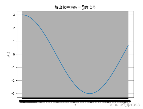
样本重建信号

拟合正弦波

    def test_reconstruction_fitting(self):
        t = np.arange(0, 2 * np.pi + 0.01, 0.01)
        x = 3 * np.cos(np.pi * t / 4)

        ax = plt.axes()
        plt.title('解出频率为w=pi/4的信号')
        plt.xlabel('t')
        plt.ylabel('x(t)')

        ax.set_xticks(t)  # 在细密的网格上绘出产生的正弦信号
        plt.plot(t, x)
        plt.grid(visible=True)

        plt.savefig('data/images/sample_reconstruction_fitting.png')

在这里插入图片描述

线性与多项式内插

直线段连接样本

    def test_interpolation1(self):
        x = [5, 3, -1]
        n = list(range(0, 3))
        t = np.arange(0, 2, 0.01)

        ax = plt.axes()
        ax.set_xticks(t)
        plt.plot(n, x)
        plt.grid(visible=True)

        plt.savefig('data/images/sample_interpolation1.png')

在这里插入图片描述
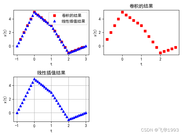
将三角形冲激响应与三个样本进行卷积

    def test_interpolation2(self):
        A = [0.2, 0.4, 0.6, 0.8, 1.0, 0.8, 0.6, 0.4, 0.2]
        B = [5, 0, 0, 0, 0, 3, 0, 0, 0, 0, -1]
        t = np.array(list(range(-4, 15)))
        Z = scipy.signal.convolve(A, B)

        vv = [0, 5, 3, -1, 0]
        xx = np.array(list(range(-1, 4)))
        xq = np.arange(-1, 3 + 0.1, 0.1)
        f = scipy.interpolate.interp1d(xx, vv, kind='linear')
        vq = f(xq)

        plt.subplot(2, 2, 1)
        plt.plot(t / 5, Z, 'rs', xq, vq, 'b^')
        # 绘出卷积的结果和线性插值的结果，分别用红色和蓝色表示
        plt.xlabel('t')
        plt.ylabel('x(t)')
        plt.legend(['卷积的结果', '线性插值结果'])
        plt.subplot(2, 2, 2)
        plt.plot(t / 5, Z, 'rs')  # 绘出卷积的结果
        plt.title('卷积的结果')
        plt.xlabel('t')
        plt.ylabel('x(t)')
        plt.subplot(2, 2, 3)
        plt.plot(xq, vq, 'b^')  # 线性插值的结果
        plt.title('线性插值结果')
        plt.xlabel('t')
        plt.ylabel('x(t)')
        plt.grid(visible=True)

        plt.tight_layout()
        plt.savefig('data/images/sample_interpolation2.png')

在这里插入图片描述
将这三个数据点拟合为二阶多项式

    def test_polynomial_interpolation(self):
        x = [5, 3, -1]
        n = np.array(list(range(0, 3)))
        p = np.polyfit(n, x, 2)
        nn = np.arange(-5, 5 + 0.5, 0.5)
        f = np.polyval(p, nn)
        t = np.arange(-5, 5 + 0.1, 0.1)

        ax = plt.axes()
        plt.legend(['样本点二阶多项式拟合结果'])
        plt.xlabel('t')
        ax.set_xticks(t)
        plt.plot(n, x, 'o', nn, f)

        plt.grid(visible=True)

        plt.savefig('data/images/polynomial_interpolation.png')

在这里插入图片描述

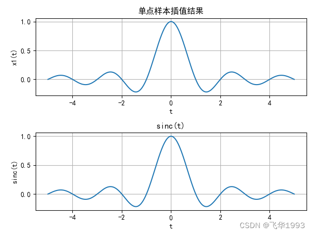
理想低通滤波器

对t=0处的数值为1的单点样本进行插值，绘出大约从-5到5的结果。它应该和sinc函数形状相一致。

    def test_low_pass_filter1(self):
        t = np.arange(-5, 5 + 0.01, 0.01)
        x1 = np.sinc(t)

        plt.subplot(2, 1, 1)
        plt.plot(t, x1)
        plt.title('单点样本插值结果')
        plt.xlabel('t')
        plt.ylabel('x1(t)')
        plt.grid(visible=True)

        plt.subplot(2, 1, 2)
        plt.plot(t, np.sinc(t))
        plt.title('sinc(t)')
        plt.xlabel('t')
        plt.ylabel('sinc(t)')
        plt.grid(visible=True)

        plt.tight_layout()
        plt.savefig('data/images/low_pass_filter1.png')

在这里插入图片描述
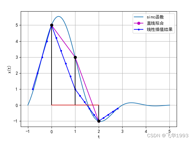
对 $x_a(t)\overset{\infty}{\underset{n=-\infty}{\Sigma}}x_a(nt)\frac{\sin(\pi(t-nT_s)/T_s)}{\pi(t-nT_s)/T_s}$ 给定及实验内容中的三点情形进行插值。

    def test_low_pass_filter2(self):
        xn = np.array([5, 3, -1])
        M = 0
        N = 2
        n = np.array(list(range(M, N + 1)))
        Ts = 1
        t1 = np.arange(-1, 5 + 0.05, 0.05)
        xa = np.matrix(xn) * np.matrix(np.sinc(np.array(
            np.matrix(1 / Ts * (np.ones([len(n), 1])) * np.matrix(t1)) - np.array(
                np.matrix(n).T * np.matrix(Ts) * np.matrix(np.ones([1, len(t1)]))))))
        xa = np.array(xa)[0]
        # 基于（3.18）的内插表达式
        x = [5, 3, -1]  # 直线段的转折点
        n = np.array(list(range(0, 3)))
        A = [0.2, 0.4, 0.6, 0.8, 1.0, 0.8, 0.6, 0.4, 0.2]  # 冲激响应
        B = [5, 0, 0, 0, 0, 1, 0, 0, 0, 0, -1]
        tt = np.array(list(range(-4, 15)))
        C = scipy.signal.convolve(A, B)  # 计算线性插值

        plt.xlabel('t')
        plt.ylabel('x(t)')  # 拟合正弦波
        plt.plot(t1, xa, n, x, 'o-m', tt / 5, C, '.-b')
        # 将直线段与正弦波进行拟合，其中直线拟合用洋红色曲线来表示，线性插值结果用蓝色曲线来表示
        plt.stem(range(M, N + 1), xn, 'k')
        plt.legend(['sinc函数', '直线拟合', '线性插值结果'])
        plt.grid(visible=True)

        plt.savefig('data/images/low_pass_filter2.png')