


1.numpy介绍
1.1.简介
- Numpy(Numerical Python)是一个开源的Python 科学计算库 ,用于快速处理任意维度的数组。
- Numpy支持常见的数组和矩阵操作。对于同样的数值计算任务,使用Numpy比直接使用Python要简洁的多。
- Numpy使用ndarray对象来处理多维数组,该对象是一个快速而灵活的大数据容器。
1.2.ndarray
numpy提供一个ndarray对象来存储一个任意维度的数组。简单创建一个ndarray对象:
import numpy as np

score = np.array(
[[80, 89, 86, 67, 79],
[78, 97, 89, 67, 81],
[90, 94, 78, 67, 74],
[91, 91, 90, 67, 69],
[76, 87, 75, 67, 86],
[70, 79, 84, 67, 84],
[94, 92, 93, 67, 64],
[86, 85, 83, 67, 80]]
)
1.3.与python数组效率对比
import random
import time
import numpy as np
a = []
for i in range(100000000):
    a.append(random.random())

# 通过%time魔法方法, 查看当前行的代码运行一次所花费的时间
%time sum1=sum(a)

b=np.array(a)

%time sum2=np.sum(b)
输入如下:
CPU times: user 690 ms, sys: 214 ms, total: 904 ms
Wall time: 904 ms
CPU times: user 83.6 ms, sys: 214 µs, total: 83.8 ms
Wall time: 83.6 ms
可以看到
1.4.效率分析
1.4.1.存储方式
numpy采用连续存储,每个block数据格式相同,不仅查找方便,在如矩阵相乘时也可以多个block同时计算,效率远高循环语句。

1.4.2.ndarray支持并行化运算
numpy内置了并行运算功能,当系统有多个核心时,做某种计算时,numpy会自动做并行计
1.4.3.底层使用c语言
2.N维数组-ndarray
2.1.ndarray属性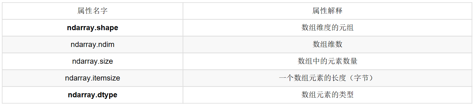
重要的是 .shape 和 .dtype ,从shape中可以看到数组有几个维度,在各个维的长度,.dtype 可以指定数组元素类型和查看类型。
2.2.ndarray.shape
这是一维数组,长度为3
a = np.array([1,2,3])
a.shape
(3,)
加一个括号,就是二位数组,第二个维度上长度为1,第一个长度为3
a = np.array([[1,2,3]])
a.shape
(1, 3)
再加一个括号就是三位数组,第三个维度长度为1,第二个维度长度为1,第三个维度长度为3,可以看出当得到一个高维数组的时候,从外到里依次找到各个维度是一个好方法。
a = np.array([[[1,2,3]]])
a.shape
(1, 1, 3)
下面观察一个复杂点的高维数组
b = np.array([[[[1, 2, 3], [4, 5, 6]]],[[[1, 2, 3],[5,6,7]]]])
print(b)
b.shape
[[[[1 2 3]
   [4 5 6]]]


 [[[1 2 3]
   [5 6 7]]]]
(2, 1, 2, 3)
有四个括号所以是四维数组
每个四括号里有两个三括号,所以第一个维度长度为2,
每个三括号里有一个二括号,所以第二个维度长度为1,
每个二括号里有两个一括号,所以第三个维度长度为2,
每个一括号里有三个数,所以第四个维度长度为3。
2.3.ndarray.dtype
ndarray数据类型如下:

创建的时候指定类型:
# 浮点数类型
b = np.array([[1, 2, 3], [4, 5, 6]], dtype=np.float32)
b
array([[1., 2., 3.],
       [4., 5., 6.]], dtype=float32)
# 字符串类型
arr = np.array(["pythonI", "hello", "I"], dtype=np.string_)
arr
# S指字符串,7指最长的字符串长度
array([b'pythonI', b'hello', b'I'], dtype='|S7')
3.基本操作
3.1.生成数组方法
3.1.1.使用ones和zeros方法
# 第一个参数指定shape,第二个参数指定类型
one = np.ones([4,8],int)
one
array([[1, 1, 1, 1, 1, 1, 1, 1],
       [1, 1, 1, 1, 1, 1, 1, 1],
       [1, 1, 1, 1, 1, 1, 1, 1],
       [1, 1, 1, 1, 1, 1, 1, 1]])
zero = np.zeros([4,8],float)
zero
array([[0., 0., 0., 0., 0., 0., 0., 0.],
       [0., 0., 0., 0., 0., 0., 0., 0.],
       [0., 0., 0., 0., 0., 0., 0., 0.],
       [0., 0., 0., 0., 0., 0., 0., 0.]])
可以直接将0全转1或者1全转0
zero1 = np.zeros_like(one)
zero1
array([[0, 0, 0, 0, 0, 0, 0, 0],
       [0, 0, 0, 0, 0, 0, 0, 0],
       [0, 0, 0, 0, 0, 0, 0, 0],
       [0, 0, 0, 0, 0, 0, 0, 0]])
3.1.2.拷贝
a = np.array([[1, 2, 3], [4, 5, 6]])
a1 = np.array(a)
a2 = np.asarray(a)
print(a1)
print(a2)
[[1 2 3]
 [4 5 6]]
[[1 2 3]
 [4 5 6]]
区别是a1分配另一个存储地址,a2只想a的存储地址
a[0][0] = 100
print(a)
print(a1)
print(a2)
[[100   2   3]
 [  4   5   6]]
[[1 2 3]
 [4 5 6]]
[[100   2   3]
 [  4   5   6]]
3.1.3.生成固定范围数组
3.1.3.1.指定两头,指定数量
线性
np.linspace(0, 100, 7)
array([  0.        ,  16.66666667,  33.33333333,  50.        ,
        66.66666667,  83.33333333, 100.        ])
指数
np.logspace(0, 2, 4)
array([ 1. , 4.64158883, 21.5443469 , 100. ])
3.1.3.2.指定两头,指定步长
np.arange(0,100,2)
array([ 0,  2,  4,  6,  8, 10, 12, 14, 16, 18, 20, 22, 24, 26, 28, 30, 32,
       34, 36, 38, 40, 42, 44, 46, 48, 50, 52, 54, 56, 58, 60, 62, 64, 66,
       68, 70, 72, 74, 76, 78, 80, 82, 84, 86, 88, 90, 92, 94, 96, 98])
3.1.4.生成随机数组
3.1.4.1.正太分布
x1 = np.random.normal(0, 1, 100000000)
x1
array([ 0.49987683, -0.07768792,  1.68092843, ...,  1.09855313,
       -1.47816434, -0.80185882])
3.1.4.1.均匀分布
随机生成元素在-1到1之间的多维数组
第三个参数可以给一个整数n,表示[n,1]
np.random.uniform(-1,1,[4,3])
array([[ 0.63270773, -0.0282482 ,  0.90389324],
       [ 0.36848579,  0.10458935, -0.90177607],
       [ 0.66366539,  0.61581464,  0.1457086 ],
       [ 0.76395906, -0.50348758, -0.66971391]])
随机生成元素在-10到10之间的整数的多维数组
np.random.randint(-10,10,[4,3])
array([[ 8,  8, -6],
       [ 0, -9,  0],
       [-5,  8, -1],
       [-8,  3,  6]])
3.2.数组的索引,切片
索引的法则同找某一个元素是一样的,区别是定位前两个后最后一个是一个范围内多个元素(定位某一个相当于[x1,x2,a:a+1]。
a1 = np.array([ [[1,2,3,4],[4,5,6,7]], [[12,3,34,45],[5,6,7,23]]])
a1[0,0,1:3]
array([2, 3])
3.3.形状修改
3.3.1.ndarray.reshape()
a = np.array([[  2,   1,  -2],
       [  0,  -4,  -1],
       [  3, -10,  -2],
       [  5, -10,  -8]])
a.reshape(3,4)
array([[  2,   1,  -2,   0],
       [ -4,  -1,   3, -10],
       [ -2,   5, -10,  -8]])
ndarray.reshape()有一个优势是行数列数可以只指定一个,但是另外一个必须是整数,即size得被指定的那个数除尽,否则会报错。ndarray.resize()就没这个功能。
a.reshape(2,-1)
array([[  2,   1,  -2,   0,  -4,  -1],
       [  3, -10,  -2,   5, -10,  -8]])
3.3.2.ndarray.resize()
a.resize(2,6)
a
array([[  2,   1,  -2,   0,  -4,  -1],
       [  3, -10,  -2,   5, -10,  -8]])
这是这三个变形中唯一一个改变数组本身的方法。
3.3.3.ndarray.T
a.T
array([[  2,   0,   3,   5],
       [  1,  -4, -10, -10],
       [ -2,  -1,  -2,  -8]])
3.4.类型修改
3.4.1.nparray.astype()
x1 = np.random.uniform(-5,5,[4,3])
x1
array([[ 3.17261349, -1.67454024,  2.05741141],
       [-0.57314672,  1.81570025,  4.46254308],
       [-0.87152285, -0.02815763, -1.6252102 ],
       [ 4.26739991, -3.77447017,  2.30158367]])
x2 = x1.astype(np.int32)
x2
array([[ 3, -1,  2],
       [ 0,  1,  4],
       [ 0,  0, -1],
       [ 4, -3,  2]])
3.4.2.nparray.tobytes()()
转成字符串
x2.tobytes()
b'\x03\x00\x00\x00\xff\xff\xff\xff\x02\x00\x00\x00\x00\x00\x00\x00\x01\x00\x00\x00\x04\x00\x00\x00\x00\x00\x00\x00\x00\x00\x00\x00\xff\xff\xff\xff\x04\x00\x00\x00\xfd\xff\xff\xff\x02\x00\x00\x00'
3.5.数组去重
3.5.1.np.unique()
x = np.array([[1,2,3,4],[3,4,5,6]])
y = np.unique(x)
print(x)
print("去重后...")
print(y)
[[1 2 3 4]
 [3 4 5 6]]
去重后...
[1 2 3 4 5 6]
4.ndarray运算
4.1.逻辑运算
score = np.random.randint(40, 100, (10, 5))
test_score = score[6:,0:5]
print("score=\n",score)
print("test_score=\n",test_score)
print("test_score>60\n",test_score>60)
test_score[test_score > 60] = 1
print("test_score=\n",test_score)
score=
 [[98 46 98 40 60]
 [68 84 68 56 77]
 [59 75 56 92 77]
 [92 91 56 48 66]
 [49 44 42 56 83]
 [44 44 62 88 63]
 [53 66 91 72 75]
 [78 41 56 67 73]
 [83 42 99 53 50]
 [93 87 75 54 83]]
test_score=
 [[53 66 91 72 75]
 [78 41 56 67 73]
 [83 42 99 53 50]
 [93 87 75 54 83]]
test_score>60
 [[False  True  True  True  True]
 [ True False False  True  True]
 [ True False  True False False]
 [ True  True  True False  True]]
test_score
 [[53  1  1  1  1]
 [ 1 41 56  1  1]
 [ 1 42  1 53 50]
 [ 1  1  1 54  1]]
4.2.逻辑运算
# 判断前两名同学的成绩[0:2, :]是否全及格
np.all(score[0:2, :] > 60)
False
判断前两名同学的成绩[0:2, :]是否有大于90分的
np.any(score[0:2, :] > 80)
True
4.3.np.where(三元运算符)
# 随机生成10名同学的5门成绩
score = np.random.randint(40, 100, (10, 5))
# 获取前四名同学的前四们成绩
fourstudents = score[:4, :4]
# 判断这四名同学各科是否及格,及格为1,不及格为0
ifPass = np.where(fourstudents > 60, 1, 0)
print(ifPass)
# 并不改变原数组
print(fourstudents)
[[1 1 1 1]
 [1 1 1 1]
 [0 1 0 1]
 [1 1 0 1]]
[[85 79 69 83]
 [64 93 80 67]
 [46 72 55 77]
 [72 97 60 66]]
np.where的第一个参数可以是任何逻辑判断语句,numpy为我们提供了专门的and和or方法 np.logical_and, np.logical_or
np.where(np.logical_and(fourstudents> 60, fourstudents< 90), 1, 0)
array([[1, 1, 1, 1],
       [1, 0, 1, 1],
       [0, 1, 0, 1],
       [1, 0, 0, 1]])
4.4.统计运算
进行统计的时候,axis 轴的取值并不一定,Numpy中不同的API轴的值都不一样,在这里,axis 0代表列, axis 1代表行去进行统计
常见的api见下图即可,一看就懂

5.数组间运算
5.1.数组与数计算
arr = np.array([[1,2,3,4],
               [2,3,4,5]])
print("arr+1=\n",arr+1)
print("arr*2=\n",arr*2)
arr+1=
 [[2 3 4 5]
 [3 4 5 6]]
arr*2=
 [[ 2  4  6  8]
 [ 4  6  8 10]]
5.2.数组与数组的运算
数组shape相等可以直接计算,shape不等时满足广播的规则也可以计算
5.2.1.广播机制
满足了以下任意一条即可运算
- 两个数组的后缘维度(trailing dimension,即从末尾开始算起的维度)的轴长度相符
- 其中的一方的长度为1
比如这样子可以,从后往前看虽然每个维度的长度都不同,但是都能找到1
arr1 = np.random.randint(-10,10,[4,1])
arr2 = np.random.randint(-10,10,[1,3])
arr1+arr2
array([[11,  5, 17],
       [ 4, -2, 10],
       [-2, -8,  4],
       [ 6,  0, 12]])
这样子也可以
arr1 = np.random.randint(-10,10,[4,1])
arr2 = np.random.randint(-10,10,[4,3])
arr1+arr2
但是这样子就会报错了,第二个维度长度不相同,且没有1
arr1 = np.random.randint(-10,10,[4,1])
arr2 = np.random.randint(-10,10,[2,3])
arr1+arr2
ValueError                                Traceback (most recent call last)
~\AppData\Local\Temp\ipykernel_28360\1465271764.py in <module>
      1 arr1 = np.random.randint(-10,10,[4,1])
      2 arr2 = np.random.randint(-10,10,[2,3])
----> 3 arr1+arr2

ValueError: operands could not be broadcast together with shapes (4,1) (2,3)
4.6.矩阵
矩阵,英文matrix,和array的区别矩阵必须是2维的,但是array可以是多维的。
矩阵的运算有两个api: np.matmul(a,b) 和 np.dot(a,b),两者的区别是 np.matmul()不能进行矩阵与标量相乘运算,np.dot()可以。
a = np.array([[80, 86],
[82, 80],
[85, 78],
[90, 90],
[86, 82],
[82, 90],
[78, 80],
[92, 94]])
b = np.array([[0.7], [0.3]])
# 意义是平时分占7成,期末占3成,妥妥的水课
np.dot(a,b)
array([[800, 860],
       [820, 800],
       [850, 780],
       [900, 900],
       [860, 820],
       [820, 900],
       [780, 800],
       [920, 940]])


 2229
2229

 被折叠的 条评论
为什么被折叠?
被折叠的 条评论
为什么被折叠?
 到【灌水乐园】发言


