【图像处理】RGB图像边缘检测

【fishing-pan：https://blog.csdn.net/u013921430 转载请注明出处】

灰度图边缘检测

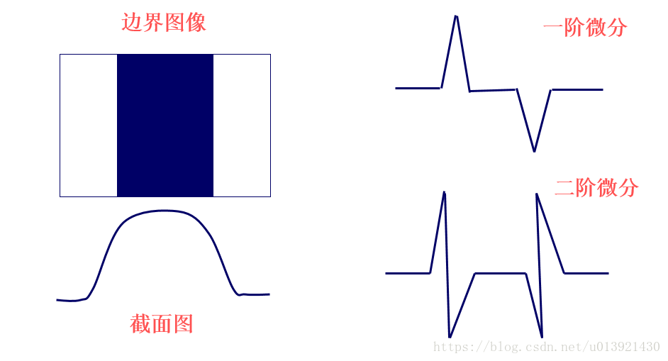
   在学习图像处理时，首先接触到的就是灰度图像的边缘检测，这是图像处理最基础的也是最重要的一环，熟悉图像边缘检测有助于我们学习其他的数字图像处理方法。由于图像的边缘区域会存在明显的像素值阶跃，因此边缘检测主要是通过获得图像灰度梯度，进而通过梯度大小和变化来判断图像边缘的。
  

   因此，我们可以通过一阶差分；
$$\begin{gathered} \Delta f_x(x,y)=f(x+1,y)-f(x,y) \\ \Delta f_y(x,y)=f(x,y+1)-f(x,y) \end{gathered}$$
   或者二阶差分对边缘区域进行判断；
$$\begin{gathered} \Delta f_{xx}(x,y)=f(x+1,y)+f(x-1,y)-2f(x,y) \\ \Delta f_{yy}(x,y)=f(x,y+1)+f(x,y-1)-2f(x,y) \end{gathered}$$
   其中一阶差分可以判断边缘是否存在，二阶差分还可以根据正负号判断像素点在图像边缘亮的一侧还是暗的一侧。
   其他的边缘检测方法还包括一些梯度算子，例如Prewitt算子、Sobel算子，Canny算子，LOG边缘检测算子等，在此不做说明。

彩色图边缘检测

   RGB 图像使用三个通道存储像素信息，我们可以将这三个通道的信息看作是一个矢量，而矢量是不存在梯度的概念的，我们无法直接将上诉方法或算子直接用于RGB 图像，而且RGB图像单个通道的梯度信息又无法反映整体的梯度信息。
   在《数字图像处理》（冈萨雷斯）中提到了一种针对彩色图像的边缘检测方法，这种方法由 Di Zenzo 等人在1986年提出，下面就一起看看这种方法如何得出。

Di Zenzo’s gradient operator

   在图像多通道图像$f(x,y)$ 中的某一点$P(x,y)$ 处，假设其梯度方向为$\theta$
$$\Delta f=\Vert f(x+\epsilon cos\theta ,y+\epsilon sin\theta )-f(x,y)\Vert$$
   为了便于计算，将计算绝对值换为计算平方，令
$$\Delta f^2={\Vert f(x+\epsilon cos\theta ,y+\epsilon sin\theta )-f(x,y)\Vert }^2$$
   对$f(x+\epsilon cos\theta ,y+\epsilon sin\theta )$进行二元泰勒展开；
$$\begin{array}{rl}f(x+\epsilon cos\theta ,y+\epsilon sin\theta )& =f(x,y)+\sum _{i=1}^m(\epsilon cos\theta \cdot \frac{\partial f_i(x,y)}{\partial x}+\epsilon sin\theta \cdot \frac{\partial f_i(x,y)}{\partial y})+o^n\\ & \approx f(x,y)+\sum _{i=1}^m(\epsilon cos\theta \cdot \frac{\partial f_i(x,y)}{\partial x}+\epsilon \cdot sin\theta \cdot \frac{\partial f_i(x,y)}{\partial y})\end{array}$$
   其中$m$表示图像通道数目，为了方便表述使用$\frac{\partial f_i}{\partial x}$代替$\frac{\partial f_i(x,y)}{\partial x}$，而在求导时各个通道之间是相互独立的，则有；
$$\Delta f^2\approx \sum _{i=1}^m(\epsilon cos\theta \cdot \frac{\partial f_i}{\partial x}+\epsilon sin\theta \cdot \frac{\partial f_i}{\partial y}{)}^2$$
  重新定义一个函数$G(\theta )$，令
$$\begin{array}{rl}G(\theta )& =\sum _{i=1}^m(\epsilon cos\theta \cdot \frac{\partial f_i}{\partial x}+\epsilon sin\theta \cdot \frac{\partial f_i}{\partial y}{)}^2\\ & ={\epsilon }^2(cos{\theta }^2\sum _{i=1}^m{\Vert \frac{\partial f_i}{\partial x}\Vert }^2+sin{\theta }^2\sum _{i=1}^m{\Vert \frac{\partial f_i}{\partial y}\Vert }^2+2sin\theta cos\theta \sum _{i=1}^m\frac{\partial f_i}{\partial x}\frac{\partial f_i}{\partial y})\end{array}$$
   进一步舍去式子中的$\epsilon$ 项，令
$$G(\theta )=cos{\theta }^2\sum _{i=1}^m{\Vert \frac{\partial f_i}{\partial x}\Vert }^2+sin{\theta }^2\sum _{i=1}^m{\Vert \frac{\partial f_i}{\partial y}\Vert }^2+2sin\theta cos\theta \sum _{i=1}^m\frac{\partial f_i}{\partial x}\frac{\partial f_i}{\partial y}$$
   为了进一步方便表述；令
$$E=\sum _{i=1}^m{\Vert \frac{\partial f_i}{\partial x}\Vert }^2;F=\sum _{i=1}^m{\Vert \frac{\partial f_i}{\partial y}\Vert }^2;H=\sum _{i=1}^m\frac{\partial f_i}{\partial x}\frac{\partial f_i}{\partial y}$$
$$G(\theta )=cos{\theta }^{2}E+sin{\theta }^{2}F+2sin\theta cos\theta H$$
   现在$\theta$成为了式子中唯一的变量，再回到边缘的定义上，边缘的方向是图像像素梯度最大的方向。也就是说梯度的方向${\theta }_{max}$ 会使$G(\theta )$ 取最大值，则；
$${\theta }_{max}=\underset{argmax}{G(\theta )}$$
   对$G(\theta )$ 进行求导；
$$G(\theta {)}^{{}^{\prime }}=-Esin2\theta +Fsin2\theta +2Hcos2\theta$$
   令$G(\theta {)}^{{}^{\prime }}=0$，得；
$$\begin{gathered} tan2{\theta }_{max}=\frac{2H}{E-F} \\ {\theta }_{max}=\frac{1}{2}arctan(\frac{2H}{E-F}+k\pi ) \end{gathered}$$
   很明显$G(\theta )$ 是一个以$\pi$ 为周期的周期函数，如果只考虑区间$\left[0,\pi \right)$，且${\theta }_{max}$ 落到该区间内，则会有另一个让$G(\theta )$取极值的解也落在该区域内，这个值是${\theta }_{max}+\frac{\pi }{2}$或者${\theta }_{max}-\frac{\pi }{2}$。但是不论如何这两个解有一个让$G(\theta )$取极大值，另一个让其取极小值，两个角度相差 90°。
  
   说到这里大家应该都明白了，两个角度对应的方向是相互垂直的，一个是垂直于边缘的方向，也就是边缘的法向，此时梯度取最大值。另一个是平行于边缘的方向，是边缘的切向，此时梯度取极小值。
  

RGB图像的边缘检测

   在RGB图像中，$m=3$，再令；
$$\overrightarrow{u}=\frac{\partial R}{\partial x}\overrightarrow{r}+\frac{\partial G}{\partial x}\overrightarrow{g}+\frac{\partial B}{\partial x}\overrightarrow{b}$$
$$\overrightarrow{v}=\frac{\partial R}{\partial y}\overrightarrow{r}+\frac{\partial G}{\partial y}\overrightarrow{g}+\frac{\partial B}{\partial y}\overrightarrow{b}$$
   其中$\overrightarrow{r}$、$\overrightarrow{g}$、$\overrightarrow{b}$分别代表不同颜色分量的单位向量，则
$$g_{xx}=E={\overrightarrow{u}}^T\overrightarrow{u}={\Vert \frac{\partial R}{\partial x}\Vert }^2+{\Vert \frac{\partial G}{\partial x}\Vert }^2+{\Vert \frac{\partial B}{\partial x}\Vert }^2$$
$$g_{yy}=F={\overrightarrow{v}}^T\overrightarrow{v}={\Vert \frac{\partial R}{\partial y}\Vert }^2+{\Vert \frac{\partial G}{\partial y}\Vert }^2+{\Vert \frac{\partial B}{\partial y}\Vert }^2$$
$$g_{xy}=H={\overrightarrow{u}}^T\overrightarrow{v}=\frac{\partial R}{\partial x}\frac{\partial R}{\partial y}+\frac{\partial G}{\partial x}\frac{\partial G}{\partial y}+\frac{\partial B}{\partial x}\frac{\partial B}{\partial y}$$
   在利用Di Zenzo 提出的方法求得${\theta }_{max}$ 后，将以上符号带入到$G(\theta )$，可以计算出像素点梯度大小为
$$G(\theta )={\left\{\frac{1}{2}\left[(g_{xx}+g_{yy})+(g_{xx}-g_{yy})cos2{\theta }_{max}+2g_{xy}sin2{\theta }_{max}\right]\right\}}^{\frac{1}{2}}$$
   进而可以根据梯度大小进行边缘检测。

参考资料

1. S. Di Zenzo, A note on the gradient of a multi-image, Computer Vision, Graphics, and Image Processing 33 (1) (1986) 116–125.
2. 《数字图像处理》 (冈萨雷斯)