DLG:图分类

DGL : Graph Classification

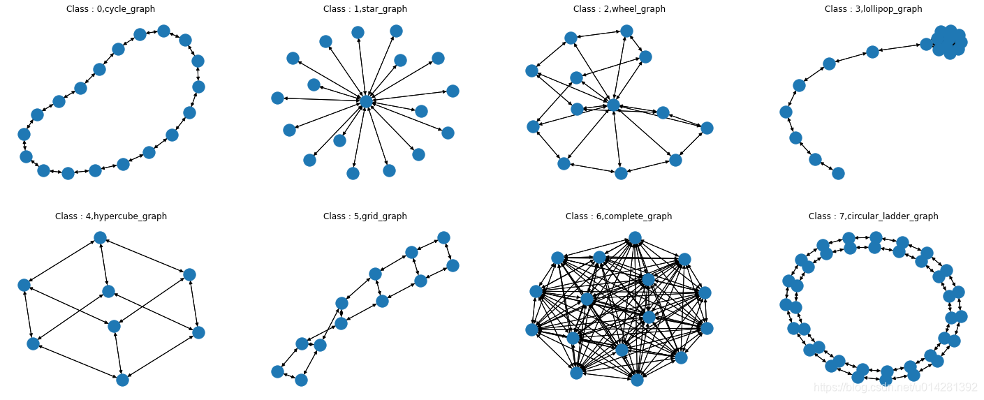
• DGL中的data.MiniGCDataset的类提供了一个合成的数据集。
• 数据集有8种不同类型的图.

load data

from dgl.data import MiniGCDataset
import matplotlib.pyplot as plt
import networkx as nx
%matplotlib inline
# 生成一个包含８０个图的数据集，每个类别十个样本
# MiniGCDataset's Parameters
# num_graphs: int,Number of graphs in this dataset.
# min_num_v: int,Minimum number of nodes for graphs
# max_num_v: int,Maximum number of nodes for graphs
dataset = MiniGCDataset(80, 8, 20)
label_names = ['cycle_graph','star_graph','wheel_graph','lollipop_graph','hypercube_graph','grid_graph','complete_graph','circular_ladder_graph']

graph visualization

plt.figure(figsize=(25, 10))
for i, index in enumerate(list(range(0, 80, 10))):
    plt.subplot(2, 4, i+1)
    graph, label = dataset[index]   # 每个类别graph的第一个图
    nx.draw(graph.to_networkx())
    plt.title('Class : %d,%s'%(label,label_names[i]))

graph mini-batch

  为了更有效地训练神经网络，通常的做法是将多个样本一起批处理。批量固定形状的张量输入非常容易（例如，批量处理两个28×28的图像，张量的形状2×28×28）。

相比之下，批处理图输入有两个挑战：

• 图很稀疏
• 图的形状不固定(节点和边的数量)

针对这个问题，DGL提供了一个dgl.batch()方法，生成batch_graphs.

• dgl.batch( cycle_graph , star_graph )

import dgl

def collate(samples):
    # The input `samples` is a list of pairs
    #  (graph, label).
    graphs, labels = map(list, zip(*samples))
    batched_graph = dgl.batch(graphs)
    return batched_graph, torch.tensor(labels)

Graph Classifier

The graph classification can be proceeded as follows:

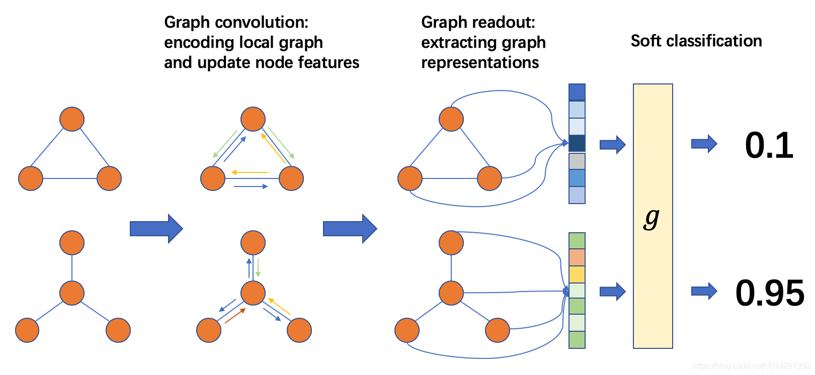
  batch graph中每个图的每个节点通过message passing/graph convolution的方式与其他节点进行“通信”，然后更新node’s feature.之后，我们用节点（和边）属性计算图的表示张量．最后，图的表示张量输入分类器g 预测图的标签。

Graph Convolution

较之前的GCN略有不同，${\sum }_{u\in \mathcal{N}(v)}$被$\frac{1}{|\mathcal{N}(v)|}{\sum }_{u\in \mathcal{N}(v)}$取代：

• $h_v^{(l+1)}=\text{ReLU}\left(b^{(l)}+{\sum }_{u\in \mathcal{N}(v)}{h}_u^{(l)}{W}^{(l)}\right)$ by
• $h_v^{(l+1)}=\text{ReLU}\left(b^{(l)}+\frac{1}{|\mathcal{N}(v)|}{\sum }_{u\in \mathcal{N}(v)}{h}_u^{(l)}{W}^{(l)}\right)$.

import dgl.function as fn
import torch
import torch.nn as nn


# Sends a message of node feature h.
msg = fn.copy_src(src='h', out='m')

def reduce(nodes):
    accum = torch.mean(nodes.mailbox['m'], 1)
    return {'h': accum}

class NodeApplyModule(nn.Module):
    """Update the node feature hv with ReLU(Whv+b)."""
    def __init__(self, in_feats, out_feats, activation):
        super(NodeApplyModule, self).__init__()
        self.linear = nn.Linear(in_feats, out_feats)
        self.activation = activation

    def forward(self, node):
        h = self.linear(node.data['h'])
        h = self.activation(h)
        return {'h' : h}

class GCN(nn.Module):
    def __init__(self, in_feats, out_feats, activation):
        super(GCN, self).__init__()
        self.apply_mod = NodeApplyModule(in_feats, out_feats, activation)

    def forward(self, g, feature):
        # Initialize the node features with h.
        g.ndata['h'] = feature
        g.update_all(msg, reduce)
        g.apply_nodes(func=self.apply_mod)
        return g.ndata.pop('h')

Readout and Classification

图的每个node的特征初始化为每个node的入度．每一次的GCN,node的入度更新为邻接node入度的均值(Rule变换)

$$h_g=\frac{1}{|\mathcal{V}|}\sum _{v\in \mathcal{V}}{h}_v$$

• func:dgl.mean_nodes:处理不同形状的图卷积后的输出

import torch.nn.functional as F


class Classifier(nn.Module):
    def __init__(self, in_dim, hidden_dim, n_classes):
        super(Classifier, self).__init__()

        self.layers = nn.ModuleList([
            GCN(in_dim, hidden_dim, F.relu),
            GCN(hidden_dim, hidden_dim, F.relu)])
        self.classify = nn.Linear(hidden_dim, n_classes)

    def forward(self, g):
        # For undirected graphs, in_degree is the same as
        # out_degree.
        h = g.in_degrees().view(-1, 1).float()
        for conv in self.layers:
            h = conv(g, h)
        g.ndata['h'] = h
        hg = dgl.mean_nodes(g, 'h')
        return self.classify(hg)

Setup and Training

• Create two dataset
• train data 400 graphs
• test data 100 graphs

import warnings
import torch.optim as optim
from torch.utils.data import DataLoader
warnings.filterwarnings('ignore')

# Create training and test sets.
trainset = MiniGCDataset(400, 10, 20)
testset = MiniGCDataset(100, 10, 20)
# Use PyTorch's DataLoader and the collate function
# defined before.
data_loader = DataLoader(trainset, batch_size=32, shuffle=True,
                         collate_fn=collate)

# Create model
model = Classifier(1, 256, trainset.num_classes)
loss_func = nn.CrossEntropyLoss()
optimizer = optim.Adam(model.parameters(), lr=0.001)
model.train()

Classifier(
  (layers): ModuleList(
    (0): GCN(
      (apply_mod): NodeApplyModule(
        (linear): Linear(in_features=1, out_features=256, bias=True)
      )
    )
    (1): GCN(
      (apply_mod): NodeApplyModule(
        (linear): Linear(in_features=256, out_features=256, bias=True)
      )
    )
  )
  (classify): Linear(in_features=256, out_features=8, bias=True)
)

epoch_losses = []
for epoch in range(150):
    epoch_loss = 0
    for iter, (bg, label) in enumerate(data_loader):
        prediction = model(bg)
        loss = loss_func(prediction, label)
        optimizer.zero_grad()
        loss.backward()
        optimizer.step()
        epoch_loss += loss.detach().item()
    epoch_loss /= (iter + 1)
    if epoch%10==0:
        print('Epoch {}, loss {:.4f}'.format(epoch, epoch_loss))
    epoch_losses.append(epoch_loss)

Epoch 0, loss 2.0452
Epoch 10, loss 1.1034
Epoch 20, loss 0.8816
Epoch 30, loss 0.7280
Epoch 40, loss 0.6544
Epoch 50, loss 0.5929
Epoch 60, loss 0.5490
Epoch 70, loss 0.4817
Epoch 80, loss 0.4273
Epoch 90, loss 0.3729
Epoch 100, loss 0.3462
Epoch 110, loss 0.3687
Epoch 120, loss 0.3651
Epoch 130, loss 0.3598
Epoch 140, loss 0.3136

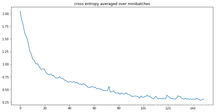
learning curve

plt.figure(figsize=(12, 6))
plt.title('cross entropy averaged over minibatches')
plt.plot(epoch_losses)

evaluated on the test

model.eval()
# Convert a list of tuples to two lists
test_X, test_Y = map(list, zip(*testset))
test_bg = dgl.batch(test_X)
test_Y = torch.tensor(test_Y).float().view(-1, 1)
probs_Y = torch.softmax(model(test_bg), 1)
sampled_Y = torch.multinomial(probs_Y, 1)
argmax_Y = torch.max(probs_Y, 1)[1].view(-1, 1)
print('Accuracy of sampled predictions on the test set: {:.4f}%'.format(
    (test_Y == sampled_Y.float()).sum().item() / len(test_Y) * 100))
print('Accuracy of argmax predictions on the test set: {:4f}%'.format(
    (test_Y == argmax_Y.float()).sum().item() / len(test_Y) * 100))

Accuracy of sampled predictions on the test set: 77.0000%
Accuracy of argmax predictions on the test set: 88.000000%

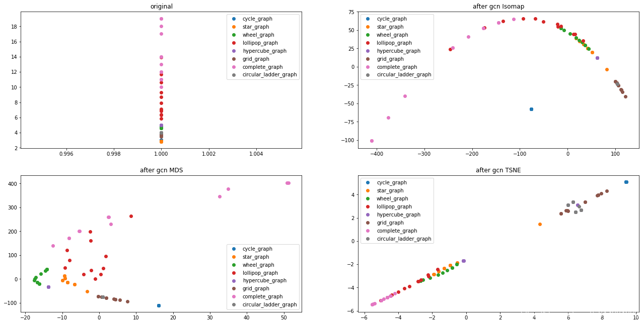
图卷积前后对比：

def get_initf(g):
    h = g.in_degrees().view(-1, 1).float()
    g.ndata['h'] = h
    hg = dgl.mean_nodes(g, 'h')
    return hg.detach().numpy()

# teat graphs features
# original features
origi_test = list(list(zip(*get_initf(test_bg).tolist()))[0])
# new features : GCNed, dgl.mean_nodes()
new_test = model.forward(test_bg).detach().numpy()
# labels list
labels = list(list(zip(*test_Y.detach().numpy().tolist()))[0])

Visualization

import numpy as np
import pandas as pd
from sklearn.manifold import Isomap, MDS, TSNE

origi_test = pd.DataFrame({'x':np.ones(100),'y':origi_test,'label':labels})

isomap = Isomap(n_components=2, n_jobs=-1)
mds = MDS(n_components=2, n_jobs=-1)
tsne = TSNE(n_components=2)

isomap_array = isomap.fit_transform(new_test)
mds_array = mds.fit_transform(new_test)
tsne_array = tsne.fit_transform(new_test)

test_isomap = pd.DataFrame({'x':isomap_array[:,0].tolist(),'y':isomap_array[:,1].tolist(),'label':labels})
test_mds = pd.DataFrame({'x':mds_array[:,0].tolist(),'y':mds_array[:,1].tolist(),'label':labels})
test_tsne = pd.DataFrame({'x':tsne_array[:,0].tolist(),'y':tsne_array[:,1].tolist(),'label':labels})

def Scatter(df):
    for i in range(8):
        temp = df[df.label == i]
        plt.scatter(temp.x, temp.y, label=label_names[i])
    plt.legend()

plt.figure(figsize=(22, 11))
for i,df,drm in zip(list(range(4)),[origi_test, test_isomap, test_mds, test_tsne],['original','after gcn Isomap','after gcn MDS','after gcn TSNE']):
    plt.subplot(2,2,i+1)
    plt.title(drm)
    Scatter(df)