行星际激波在日球层中的传播：Propagation of Interplanetary Shocks in the Heliosphere （第三部分）-CSDN博客

本文链接：https://blog.csdn.net/u014546828/article/details/147186637

Propagation of Interplanetary Shocks in the Heliosphere
[ Chapter 4 ]

本文保留原文及参考文献，参考文献详见

行星际激波在日球层中的传播：Propagation of Interplanetary Shocks in the Heliosphere （参考文献部分）-CSDN博客

Chapter 4 Analysis methods

▍4.1 Instruments ▍

In this thesis, Solar Terrestrial Relations Observatory (STEREO) A and B, Wind, Advanced Composition Explorer (ACE), and the Cluster spacecraft magnetic field and ion plasma data are used. In the following subsections, the basic descriptions of each spacecraft, its orbits, and its instruments are mentioned.

在本论文中，使用了日地关系天文台STEREO-A和STEREO-B、Wind、先进成分探测器(ACE)以及Cluster卫星的磁场和离子等离子体数据。以下小节将分别介绍各航天器的基本情况、轨道及其仪器配置。

4.1.1 The STEREO mission

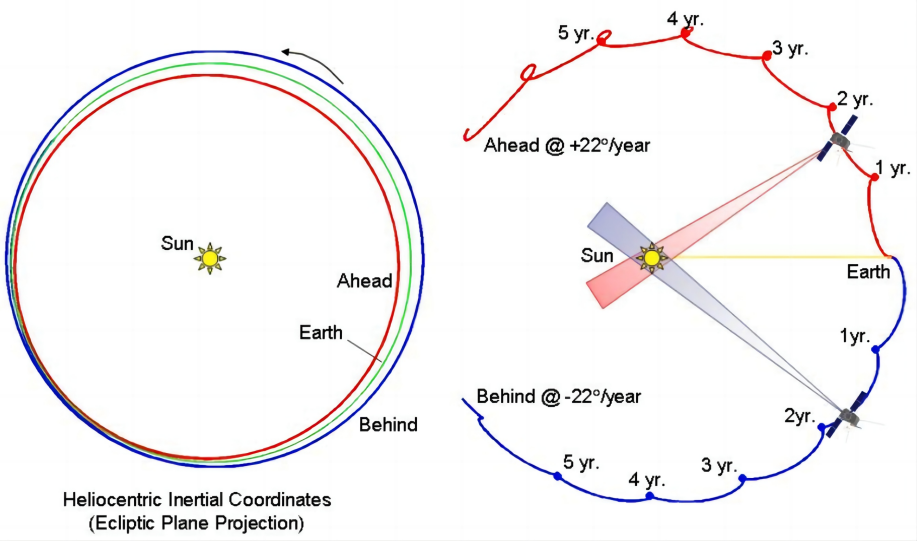
The twin Solar Terrestrial Relations Observatory (STEREO) A and B spacecraft were launched on October 26, 2006, from Kennedy Space Center (Kaiser et al., 2008). In heliospheric orbit at 1 AU, STEREO−A (Ahead) leads while STEREO−B (Behind) trails Earth. The two spacecraft separate at 44◦ from each other annually, see Figure 4.1. This formation allows the stereoscopic image of the Sun from the Sun-Earth axis angle in 3D. The purposes of the mission are to study the cause and initiation mechanisms of coronal mass ejection (CME) and their propagation through the heliosphere, discover the sites and procedures of solar energetic particles in the corona as well as the interplanetary medium, and construct a three dimensional and time-dependent model of the parameters of the solar wind (Kaiser, 2005).

双星日地关系天文台(STEREO)A和B航天器于2006年10月26日从肯尼迪航天中心发射升空(Kaiser等，2008)。在1天文单位(AU)的日球层轨道上，STEREO-A(前导)位于地球前方，而STEREO-B(后随)位于地球后方。两颗卫星每年以44°的夹角相互远离，参见图4.1。这种构型可实现从日地轴角度对太阳进行三维立体成像。该任务旨在研究日冕物质抛射(CME)的成因和触发机制及其在日球层中的传播过程，探索太阳高能粒子在日冕和行星际介质中的产生位置与过程，并建立太阳风参数的三维时变模型(Kaiser，2005)。

Figure 4.1: Left panel shows the orbits of STEREO−A and B relative to that of Earth. The right panel shows the degree of separation of two spacecraft in years from their first launch period. (Figure is from Kaiser, 2005; Figure 2)

The two spacecraft are each equipped with the complement of four scientific instruments, particularly two instruments and two instrument suites, with a total of 13 instruments on each spacecraft. The complements of the four instruments are as follows:

• 1. Sun-Earth Connection Coronal and Heliospheric Investigation (SECCHI)
• 2. STEREO/WAVES (S/WAVES)
• 3. In situ Measurements of Particles and CME Transients (IMPACT)
• 4. Plasma and Suprathermal Ion Composition (PLASTIC)

每颗STEREO卫星均配备四套科学仪器，具体包括两台独立仪器和两套仪器组，共计13台仪器。主要仪器配置如下：

• 1. 日地连接日冕和日球层调查设备 (SECCHI)
• 2. STEREO/射电与等离子体波探测仪 (S/WAVES)
• 3. 粒子与CME瞬变现场测量仪 (IMPACT)
• 4. 等离子体与超热离子成分分析仪 (PLASTIC)

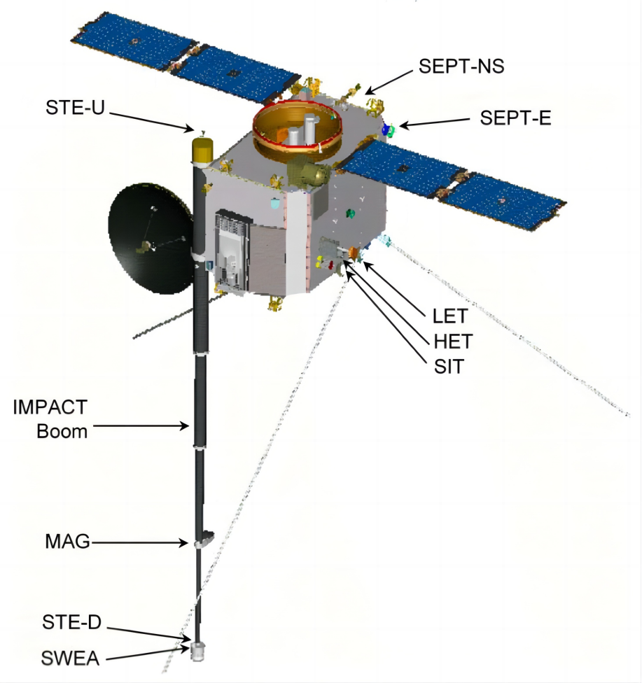
The SECCHI suite of instruments has two white light coronagraphs, an extreme ultraviolet imager, and two heliospheric white light imagers for tracking CMEs (Howard et al., 2008). The S/WAVES instrument utilizes radio waves to trace locations of the CME-driven shocks and the 3-D open field lines for the particles created by solar flares (Bougeret et al., 2008). The PLASTIC instrument measures proton, the composition of heavy ions, and alpha particles in the solar wind plasma (Galvin et al., 2008). The IMPACT suite of instruments consists of seven instruments, and three of them are located on the 6-meter boom as shown in Figure 4.2 while the others are in the main hull of the spacecraft (Acu˜na et al., 2008). The IMPACT measures protons, heavy ions, and electrons, and the MAG magnetometer sensor in it measures the in situ magnetic fields in a range of ±512nT with 0.1 nT accuracy (Kaiser and Adams, 2007).

Figure 4.2: Relative placement of the IMPACT boom on the STEREO (Figure is from Acu˜na et al., 2008; Figure 1)

Unfortunately, multiple hardware issues affecting control of the spacecraft resulted in the loss of contact with STEREO−B on October 1, 2014, (STEREO Science Center, 2018).

SECCHI仪器套件包含两台白光日冕仪、一台极紫外成像仪以及两台日球层白光成像仪，用于追踪日冕物质抛射(CME)（Howard等，2008）。

S/WAVES仪器通过无线电波来追踪CME驱动激波的位置以及太阳耀斑产生粒子的三维开放场线（Bougeret等，2008）。

PLASTIC仪器用于测量质子、重离子成分和α粒子在太阳风等离子体中的分布（Galvin等，2008）。

IMPACT仪器套件包含七台仪器，其中三台安装在6米悬臂上（如图4.2所示），其余位于航天器主舱（Acuña等，2008）。IMPACT可测量质子、重离子和电子，其搭载的MAG磁强计传感器能够以±512nT量程和0.1nT精度测量原位磁场（Kaiser和Adams，2007）。

遗憾的是，由于多重硬件故障影响航天器控制，STEREO-B于2014年10月1日失去联系（STEREO科学中心，2018）。

4.1.2 Wind

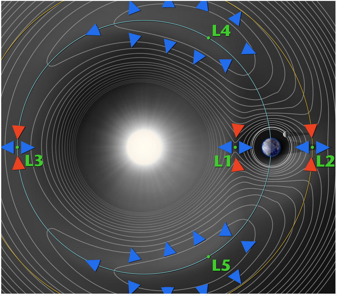
NASA's Wind spacecraft was launched on November 1, 1994, (Wilson III et al., 2021). The Wind was initially planned sent to L1 Lagrangian point but was delayed to study the magnetosphere and lunar environment. Following a sequence of orbital adjustments, the Wind spacecraft was positioned in a Lissajous orbit close to the L1 Lagrange point in early 2004 for studying the incoming solar on the verge of impacting Earth's magnetosphere (NASA WIND team, 2020), see Figure 4.3.

NASA的Wind卫星于1994年11月1日发射（Wilson III等，2021）。该卫星原计划前往拉格朗日点，后为研究磁层和月球环境推迟计划。经过一系列轨道调整，Wind卫星于2004年初进入L1拉格朗日点附近的李萨如轨道，用于研究即将影响地球磁层的太阳风（NASA WIND团队，2020），参见图4.3。

Figure 4.3: Lagrangian points in the Sun-Earth system. (Credit: NASA Solar System Exploration, 2020)

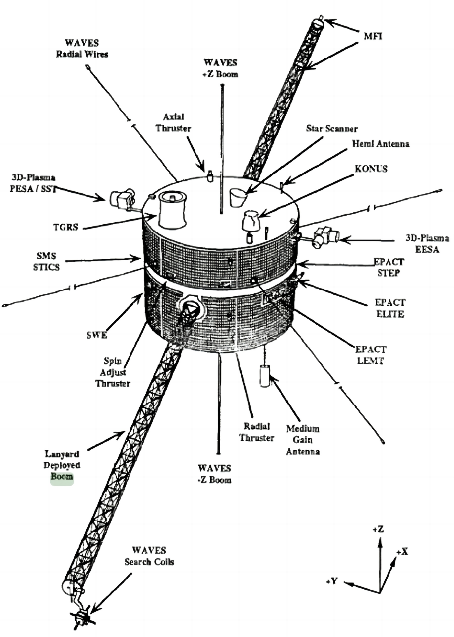
The object of the mission is to study solar wind plasma, magnetic field, and solar and cosmic energetic particles. The spacecraft is equipped with the eight instruments such as Solar Wind Experiment (SWE Ogilvie et al., 1995), 3-D plasma (3DP Wilson III, 2011), Magnetic Field Investigation (MFI Lepping et al., 1995), Solar wind/mass suprathermal ion composition studies (SMS Gloeckler et al., 1995), Energetic Particles: Composition Transport (EPACT Von Rosenvinge et al., 1995), Radio and Plasma Wave Experiment (WAVES Bougeret et al., 1995), (KONUS Mazets and Golenetskii, 1981) and Transient Gamma-Ray Spectrometer (TGRS Owens et al., 1991), see Figure 4.4.

任务目标是研究太阳风等离子体、磁场以及太阳和宇宙高能粒子。该航天器搭载了八台科学仪器，包括（详见图4.4）：

太阳风实验仪(SWE)（Ogilvie等，1995）
三维等离子体分析仪(3DP)（Wilson III，2011）
磁场探测仪(MFI)（Lepping等，1995）
太阳风/质量超热离子成分研究仪(SMS)（Gloeckler等，1995）
高能粒子成分传输仪(EPACT)（Von Rosenvinge等，1995）
射电与等离子体波实验仪(WAVES)（Bougeret等，1995）
KONUS伽马暴探测器（Mazets和Golenetskii，1981）
瞬态伽马射线光谱仪(TGRS)（Owens等，1991）

From these instruments, MFI and SWE are of interest to this thesis. The MFI consists of two magnetometers at the 12-meter boom, its measurement capability is 4 nT, 65536 nT, and measures vector magnetic field up in a time resolution of 22 or 11 vectors per second for the calibrated high-resolution data and primary science data is in time resolutions of three seconds, one minute and one hour (NASA WIND team, 2022). The SWE measures the solar wind key parameters such as velocity, density, and temperature.

本论文重点关注MFI和SWE仪器：

MFI配备两台磁强计，安装在12米悬臂上，测量范围4nT~65,536nT，可获取矢量磁场数据：
- 校准高分辨率数据：22或11矢量/秒
- 主要科学数据：3秒、1分钟和1小时分辨率（NASA WIND团队，2022）
SWE用于测量太阳风关键参数（速度、密度、温度）

Figure 4.4: Configuration of the Wind instruments. (Figure is from Harten and Clark, 1995; Figure 1)

4.1.3 ACE

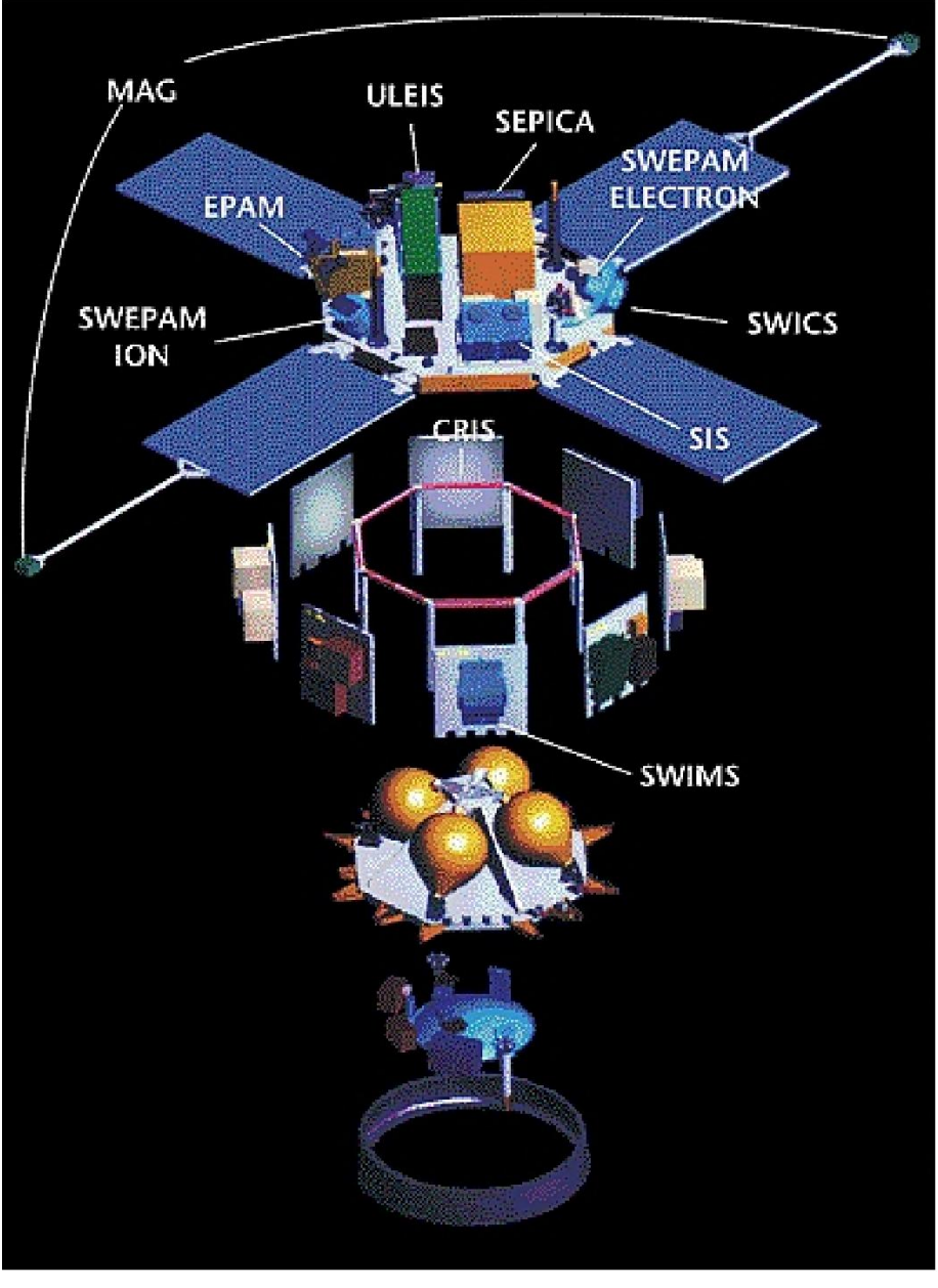
NASA's ACE spacecraft was launched on August 25, 1997, (Stone et al., 1998c). The spacecraft is located at L1 Lagrangian point same as the Wind spacecraft, see Figure 4.3. The general purposes of ACE are to gather and study particles originating from the sun, interplanetary or interstellar mediums, and the galaxy as well as to investigate the solar wind structures such as ICMEs and magnetic clouds. The spacecraft is equipped with nine primary scientific instruments and one engineering instrument such as Cosmic-Ray Isotope Spectrometer (CRIS) (Stone et al., 1998a), Electron, Proton, and Monitor (EPAM), Magnetometer (MAG) (Smith et al., 1998), Real-Time Solar Wind (RTSW) (Zwickl et al., 1998), Solar Energetic Particle Ionic Charge Analyzer (SEPICA) (Mobius et al.), Solar Isotope Spectrometer (SIS) (Stone et al., 1998b), Solar Wind Electron, Proton and Alpha Monitor (SWEPAM) (McComas et al., 1998), Solar Wind Ion Composition Spectrometer (SWICS) and Solar Wind Ion Mass Spectrometer (SWIMS) (Gloeckler et al., 1998) and Ultra-Low-Energy Isotope Spectrometer (ULEIS) (Mason et al., 1998), see Figure 4.5. The MAG consists of twin triaxial flux-gate magnetometers such that magnetometer sensors have between 3 and 6 vectors s−1 resolutions for continuous observation of the interplanetary magnetic field (Smith et 1998).

NASA ACE航天器于1997年8月25日发射升空（Stone等，1998c）。该航天器与Wind卫星同位于L1拉格朗日点（参见图4.3）。ACE的主要科学目标包括：

太阳起源粒子
分析行星际/星际介质粒子
探测银河系粒子
研究太阳风结构（ICMEs和磁云）

仪器配置（详见图4.5）：

九台主科学仪器：
1. 宇宙射线同位素光谱仪(CRIS)（Stone等，1998a）
2. 电子/质子/α粒子监测仪(EPAM)
3. 磁强计(MAG)（Smith等，1998）
4. 实时太阳风监测仪(RTSW)（Zwickl等，1998）
5. 太阳高能粒子电荷分析仪(SEPICA)（Mobius等）
6. 太阳同位素光谱仪(SIS)（Stone等，1998b）
7. 太阳风电子/质子/α粒子监测仪(SWEPAM)（McComas等，1998）
8. 太阳风离子成分光谱仪(SWICS)
9. 太阳风离子质谱仪(SWIMS)（Gloeckler等，1998）
一台工程仪器：
- 超低能同位素光谱仪(ULEIS)（Mason等，1998）

MAG磁强计技术参数：

双三轴磁通门磁强计配置
传感器分辨率：3-6矢量/秒
用于行星际磁场连续观测（Smith等，1998）

Figure 4.5: Instruments of ACE spacecraft. (Figure is from Stone et al., 1998c; Figure 6)

4.1.4 Cluster

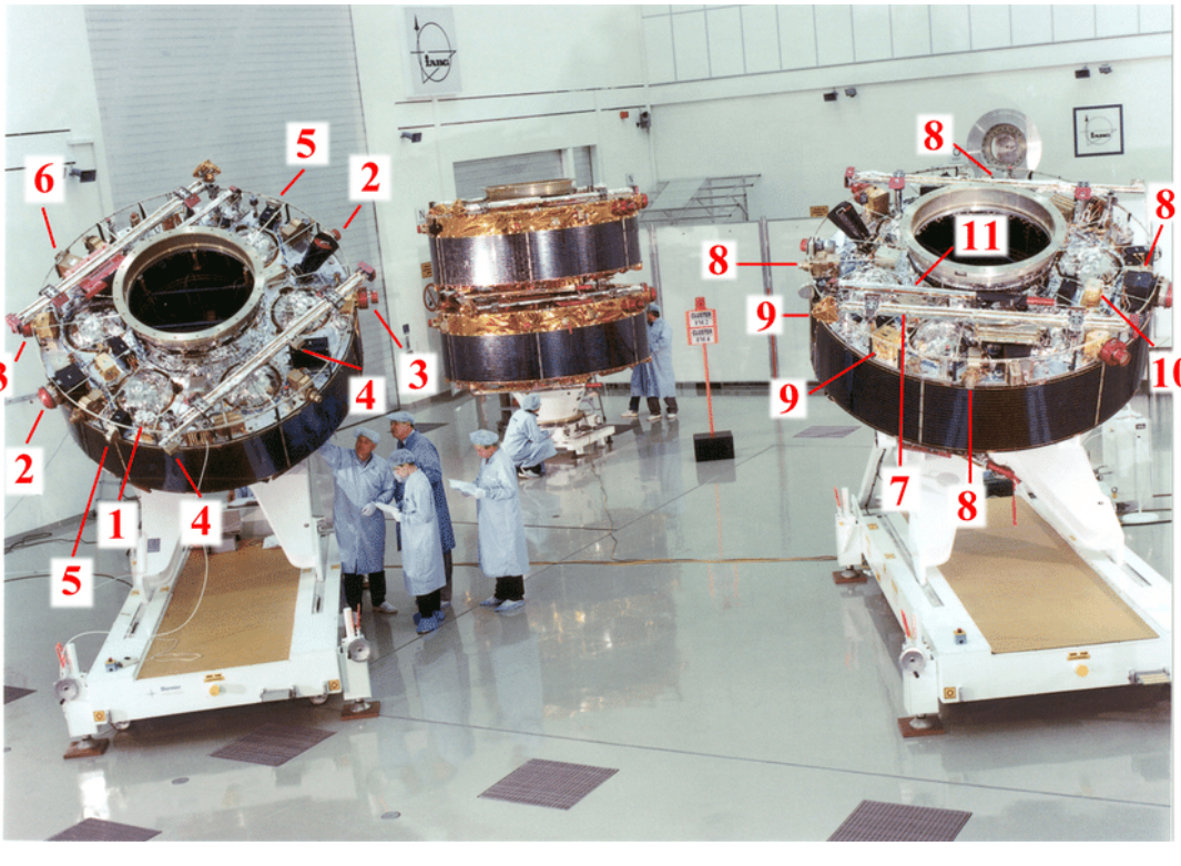
ESA's Cluster constellations consist of 4 satellites, which were launched on 16 July and 9 August 2000 (Escoubet et al., 2001). The Cluster satellites orbit in a tetrahedral formation around Earth. The orbits feature perigees close to 4 Earth radii (RE) and apogees approximately 19.6 RE away (Zhang et al., 2010). The primary objectives of the Cluster mission involve examining small-scale plasma formations and macroscopic turbulences in three dimensions in crucial plasma areas, including solar wind, bow shock, magnetopause, polar cusps, magnetotail, and auroral regions (Escoubet et al., 2001). The four satellites are each equipped with 11 instruments such as Active Spacecraft Potential Control (ASPOC) (Torkar et al., 2016), Ion Composition (CIS) (Reme et al., 1997), Electron Drift Instrument (EDI) (Haaland et al., 2007), Fluxgate Magnetometer (FGM) (Balogh et al., 1997), Plasma Electron And Current Experiment (PEACE) (Johnstone et al., 1997), Research with Adaptive Particle Imaging Detectors (RAPID) (Daly and Kronberg, 2010), Digital Wave processor (DWP) (Woolliscroft et al., 1997), Electric field and waves (EFW) (Gustafsson et al., 1997), Spatio-Temporal Analysis of Field Fluctuations (STAFF) (Cornilleau-Wehrlin et al., 1997), Wide-band plasma wave (WBD) (Gurnett et al., ), and Waves of High frequency and Sounder for Probing of Electron Density (WHISPER) (D´ecr´eau et al., 1997) as shown in Figure 4.6.

ESA的Cluster卫星星座由4颗卫星组成，分别于2000年7月16日和8月9日发射（Escoubet等，2001）。Cluster卫星采用四面体构型环绕地球运行，轨道近地点约4个地球半径(RE)，远地点约19.6 RE（Zhang等，2010）。Cluster任务的主要科学目标包括在关键等离子体区域（太阳风、弓激波、磁层顶、极尖区、磁尾和极光区）开展三维小尺度等离子体结构和宏观湍流研究（Escoubet等，2001）。

每颗卫星配备11台科学仪器（详见图4.6）：

主动航天器电位控制仪(ASPOC)（Torkar等，2016）
离子成分分析仪(CIS)（Reme等，1997）
电子漂移仪(EDI)（Haaland等，2007）
磁通门磁强计(FGM)（Balogh等，1997）
等离子体电子与电流实验仪(PEACE)（Johnstone等，1997）
自适应粒子成像探测器(RAPID)（Daly和Kronberg，2010）
数字波处理器(DWP)（Woollisc，1997）
电场与波动仪(EFW)（Gustafsson等，1997）
场波动时空分析仪(STAFF)（Cornilleau-Wehrlin等，1997）
宽频带等离子体波探测仪(WBD)（Gurnett等）
高频波与电子密度探测仪(WHISPER)（Décréau等，1997）

From the instruments, the magnetic and plasma parameters are up to our interest. Hence, the FGM magnetometer, CIS, and EFW instruments are emphasized. The Fluxgate Magnetometer (FGM) is composed of two tri-axial fluxgate magnetometers, which are installed on one of the two 5-meter radial booms. It measures in the dynamic range ±65,536nT. At the highest dynamic level, the resolution is ±8 nT, and the time resolution is 100 vectors per second (Organization, 2021). CIS (Ion composition) instrument measures three-dimensional ion distribution, and it is composed of two distinct sensors: the Composition Distribution Function (CODIF) sensor and the Hot Ion Analyzer (HIA) sensor. The CIS experiment is not operational for Cluster-2 and the HIA sensor is switched off for Cluster-4 due to a problem with the high voltage of the electrostatic analyzer (CIS team, 2021). Hence, for Cluster-2 and Cluster-4, the Electric Field and Wave (EFW) instrument measurement is useful. The EFW instrument measures the electric field fluctuations as well as the spacecraft potential, which is essential for studying plasma density and spacecraft charging.

从仪器来看，磁场和等离子体参数是关注的重点。因此，FGM磁力计、CIS和EFW仪器被重点强调。磁通门磁力计（FGM）由两个三轴磁通门磁力计组成，安装在两根5米径向伸杆的其中一根上。其测量范围为±65,536 nT。在最高动态范围下，分辨率为±8 nT，时间分辨率为每秒100个矢量（Organization, 2021）。

CIS（离子成分）仪器用于测量三维离子分布，由两个不同的传感器组成：成分分布函数（CODIF）传感器和热离子分析仪（HIA）传感器。CIS实验在Cluster-2上未运行，且由于静电分析仪的高压问题，Cluster-4的HIA传感器已关闭（CIS团队, 2021）。因此，对于Cluster-2和Cluster-4，电场与波动（EFW）仪器的测量数据非常有用。

EFW仪器可测量电场波动以及航天器电位，这对研究等离子体密度和航天器充电至关重要。

Figure 4.6: Instruments on Cluster satellites. ASPOC (1), CIS (2), EDI (3), FGM (4), PEACE (5), RAPID (6), DWP (7), EFW (8), STAFF (9), WBD (10), WHISPER (11) (Figure is from Escoubet et al., 2001; Figure 3)

▍4.2 Methods ▍

The following two methods are suitable for single-spacecraft measurements and both of them are based on the divergence of the magnetic field, ∇ · B = 0, constraint, and both of them use solely magnetic field data. The following formalization, descriptions, and derivations are based on (Sonnerup and Scheible, 1998) and (Paschmann and Daly, 2000).

以下两种方法适用于单航天器测量，均基于磁场散度∇·B=0的约束条件，且仅使用磁场数据。以下公式推导和描述基于(Sonnerup and Scheible, 1998)和(Paschmann and Daly, 2000)的研究。

4.2.1 Minimum Variance Analysis

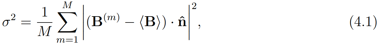
The Minimum variance analysis technique was first developed by (Sonnerup and Cahill Jr, 1967). It is based on the assumption that variations in the magnetic field would be observed when a single spacecraft passes through a 1-D current layer or wavefront. Remembering the divergence of the magnetic field constraint, ∇ · B = 0, such that the normal component of the magnetic field must remain constant. If such a normal direction can be found, then the variations in the magnetic field are zero or at the least has a minimum variance. Thus, ˆn can be determined by the minimization of the following equation:

where B^(m) ,(m = 1, 2, 3...M) is the magnetic field in a series data and B is the average magnetic field.

4.2.1 最小方差分析法

最小方差分析技术最初由Sonnerup和Cahill Jr（1967）提出。该方法基于以下假设：当单个航天器穿过一维电流层或波前时，可以观测到磁场变化。根据磁场散度约束条件∇·B=0，磁场的法向分量必须保持恒定。若能找到这样的法线方向，则磁场变化为零或具有最小方差。因此，法向量ˆn可通过最小化以下方程确定：

其中B^(m)（m=1,2,3...M）是时间序列中的磁场数据，B是平均磁场。

Taking the account of the normalization constraint |ˆn|² = 1, on which minimization is conditioned, and introducing a Lagrange multiplier, λ, for utilizing the constraint, the solution of three homogeneous linear equations can be found. The three homogeneous equations are:

where σ² is given by 4.1 and ˆn is expressed in its three components, which are along X, Y Z coordinates.

在考虑归一化约束条件|ˆn|²=1的基础上（该条件是最小化过程的前提条件），通过引入拉格朗日乘子λ来应用该约束条件，可以求解得到三个齐次线性方程的解。

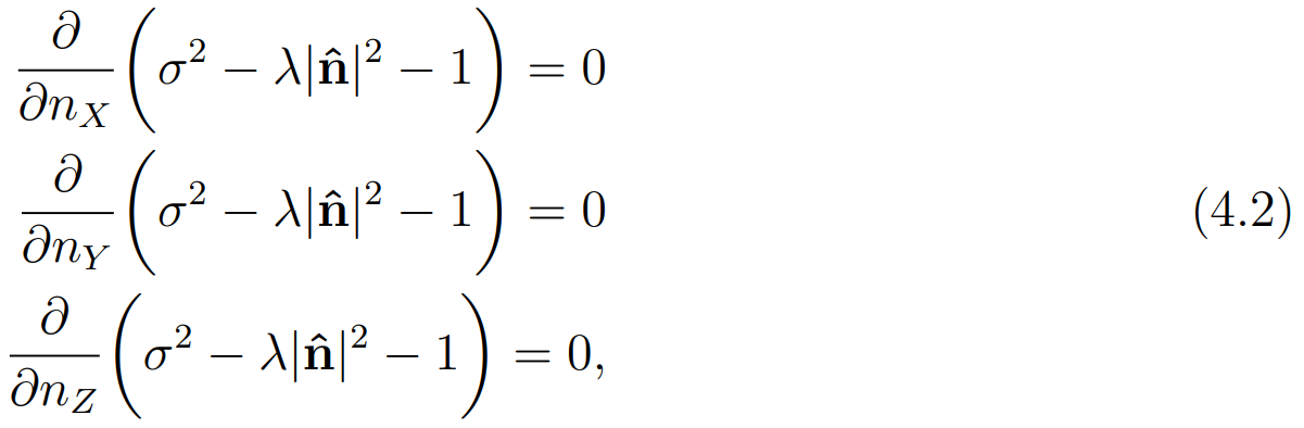
式中 σ² 由式4.1给出，ˆn 用其沿 X、Y、Z 坐标的三个分量表示。

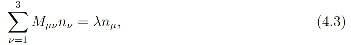
After the differentiation procedures of 4.2 are done, the resulting sets of equations can be written in matrix form:

where the subscripts µ and ν indicate cartesian coordinates and M_µν is the magnetic variance matrix:

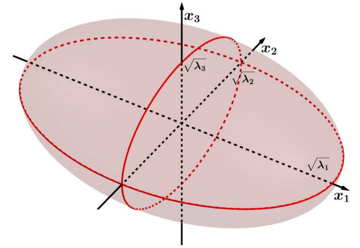
with λ being the eigenvalues with three possible values λ₁, λ₂, and λ₃ with decreasing order. The eigenvalues have their corresponding eigenvectors x₁, x₂, and x₃ of the matrix where they represent the directions of maximum, intermediate, and minimum variance of the magnetic field component. The eigenvectors corresponding to the smallest value of the λ eigenvalues are the shock normal vectors. The eigenvalue ratios, especially intermediate to minimum eigenvalue ratio, must be greater than 2 or 3 to keep the variance space ellipsoid (Paschmann and Daly, 1998) as shown in Figure 4.7.

在完成对式4.2的微分运算后，所得方程组可表示为矩阵形式：

其中下标μ和ν表示笛卡尔坐标，M_μν为磁方差矩阵：

特征值λ有三个可能值λ₁、λ₂和λ₃（按降序排列），对应的特征向量x₁、x₂和x₃分别表示磁场分量的最大、中间和最小方差方向。与最小λ值对应的特征向量即为激波法向量。为保持方差空间椭球的有效性（Paschmann和Daly，1998，参见图4.7），特征值比值（特别是中间与最小特征值之比）必须大于2或3。

Figure 4.7: The illustration of the variance space ellipsoid geometry (Figure is from Rosa Oliveira et al., 2020; Figure 1)

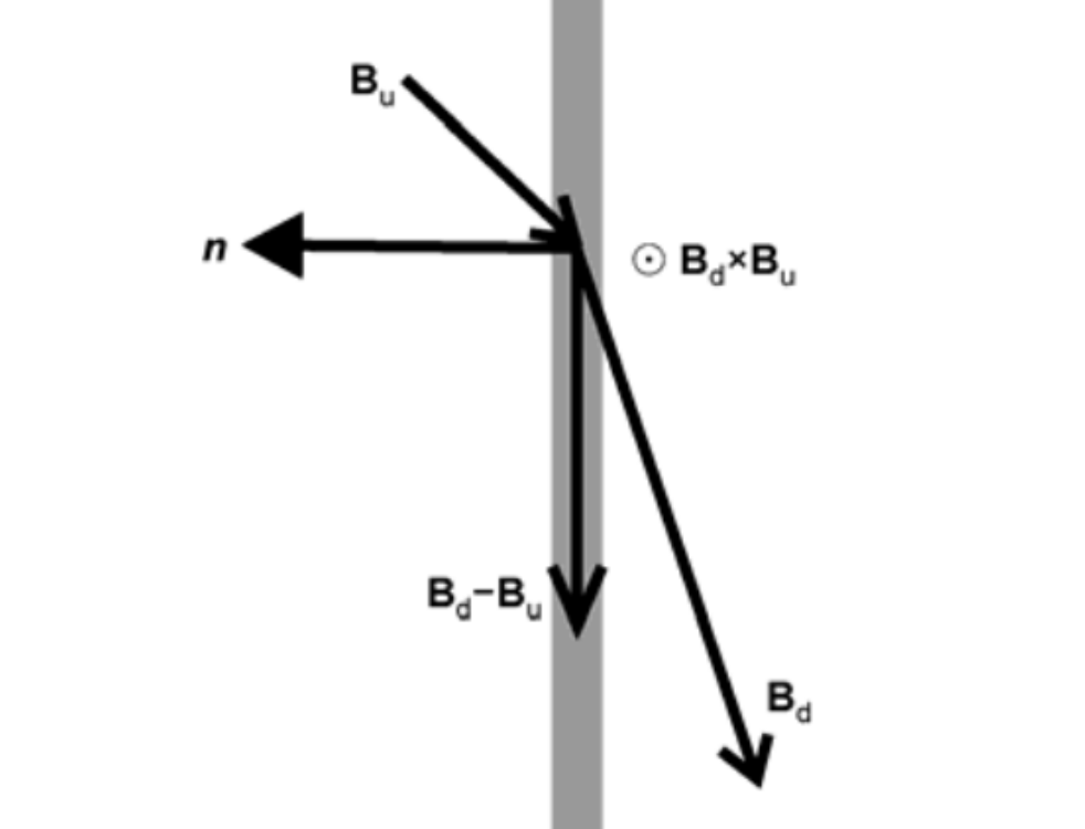
4.2.2 The Magnetic Coplanarity Method

If two vectors that lie inside a coplanar surface can be determined, the normal to the coplanar surface can be found.

The coplanarity methods are based on the magnetic coplanarity theorem, which stated that both sides of the magnetic field vectors on the shock and the shock normal lie in the same plane. Similarly, the velocity on both sides or, in other words, the velocity jump through the shock also lie in the same plane. The upstream and downstream magnetic fields and velocities satisfy the Rankine-Hugoniot conditions. So, there are multiple vectors lie in the shock plane, and the resulting constraint equations are as follows:

where the indexes up and down denote upstream and downstream, respectively.

4.2.2 磁共面性方法

若能确定位于共面表面内的两个向量，则可求出该共面表面的法向量。

磁共面性方法基于磁共面性定理，该定理指出：激波两侧的磁场向量与激波法向量同一平面内。类似地，激波两侧的速度（或称穿越激波的速度跃变）也位于同一平面。上游和下游的磁场及速度满足Rankine-Hugoniot条件，因此有多个向量位于激波平面内，由此得到的约束方程**如下：

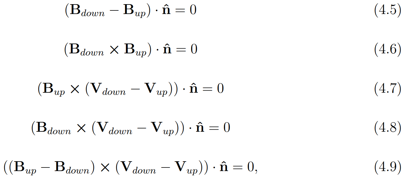
其中下标up和down分别表示上游和下游。

From 4.5 and 4.6 the magnetic coplanarity normal is defined:

where the signs are arbitrary.

The magnetic coplanarity schematic illustration is shown in Figure 4.8.

由式4.5和式4.6可定义磁共面性法向量：

式中符号可任意选取。

磁共面性示意图见图4.8。

Figure 4.8: The illustration of the magnetic coplanarity. The gray vertical line represents the shock layer. (Figure is from Shan et al., 2013; Figure 1)

Similarly, from 4.7, 4.8 and 4.9 the mixed modes for normals can be defined, respectively.

From these, the equation 4.10 is used and as denoted further on as (CP). The method of magnetic coplanarity is straightforward to implement and, as previously mentioned, it only necessitates the use of a magnetic field data (Paschmann and Daly, 1998).

类似地，根据式4.7、4.8和4.9可分别定义混合模式法向量：

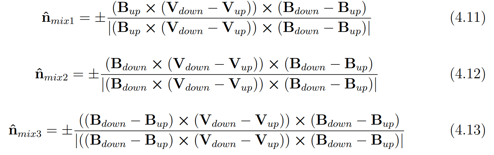
其中式4.10被采用并在后文中标记为(CP)。磁共面性方法实施简便，且如前所述仅需使用磁场数据即可完成分析（Paschmann和Daly，1998）。

4.2.3 The Utilization of the Methods

By comparing the two methods, the upstream and downstream time intervals of the magnetic field measurements are set. In this thesis work, as stated before the magnetic coplanarity method 4.10 is used out of thelanarity methods.

To accept the intervals, there are some criteria to be put in such as:

• The angle between the vectors defined by the minimum variance analysis (MVA) and the magnetic coplanarity method must be less than 15° (Facskó et al., 2008, 2009, 2010)

• The ratio between the intermediate eigenvalue and the smallest eigenvalue should be greater than 2 (Facskó et al., 2008, 2009, 2010), the same for more data points and greater than 10 for data points less than 50 Sonnerup and Cahill Jr (1967) or the ratio between the smallest eigenvalue to the intermediate eigenvalue should be smaller than 1/3 (Shan et al., 2013), which is in reverse means greater than 3.

4.2.3 方法应用
通过比较两种方法，设定了磁场测量的上游和下游时间区间。本论文选用磁共面性方法（式4.10）作为分析方法。

确定有效区间需满足以下判定准则：

角度准则
由最小方差分析法(MVA)和磁共面性方法确定的向量间夹角必须小于15°（Facskó等，2008,2009,2010）
特征值比准则

中间特征值与最小特征值之比应大于2（Facskó等，2008,2009,2010）
数据点较多时保持相同标准
数据点少于50个时，该比值需大于10（Sonnerup和Cahill Jr，1967）
或最小特征值与中间特征值之比应小于1/3（Shan等，2013），即逆向比值需大于3

4.2.4 Estimating the solar wind parameters

The following parameter estimations are based on this paper (Lumme et al., 2017)

Shock criteria

The solar wind bulk speed jump should fulfill the following conditions:

And downstream to upstream ratios should fulfill the following ratios of upstream and downstream the magnetic field, density, and temperature respectively:

激波判据：

太阳风体速度跃变需满足以下条件：

上下游比值应满足以下磁场、密度和温度的比值关系：

Shock theta:

This is the angle between the normal vector ˆn and the upstream magnetic field lines:

激波角 θ：
定义为法向量ˆn与上游磁力线之间的夹角：

Shock speed:

The shock speed in the spacecraft frame of reference:

激波速度：
在航天器参考系中的激波速度：

Upstream sound speed:

where m_p is the proton mass, T_p and T_e are proton and electron temperature. In the solar wind, the electron temperature at 1 AU is assumed to be ∼140,000 K (Newbury, 1996).

上游声速：

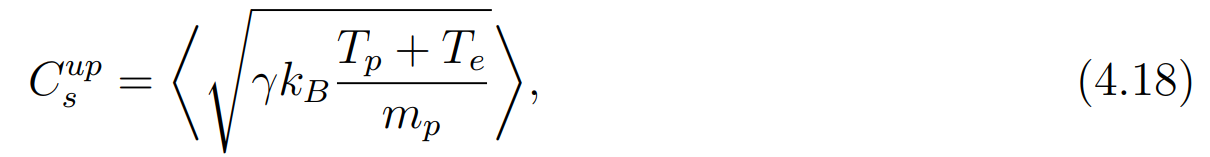
其中：m_p为质子质量；T_p和T_e分别为质子和电子温度；在1 AU处的太阳风中，电子温度假定为~140,000 K (Newbury, 1996)。

Upstream Alfvén speed:

where µ_0 is the magnetic vacuum permeability, N_p is the proton density and m_p is the proton mass.

上游阿尔芬速度：

其中：μ_0为真空磁导率；N_p为质子数密度上游磁声速；m_p 是质子质量

Upstream magnetosonic speed:

Upstream plasma beta:

Alfvén Mach number:

where V_up is the upstream velocity, V_sh is shock speed and V^up_A is the Alfvén speed. The reason for ±V_sh is a Galilean coordinate transformation to the shock rest frame. The sign ± is depend on FF shock, for which (-) or FR shock, for which (+).

上游磁声速：

上游等离子体β：

阿尔芬马赫数：

其中：V_up为上游速度；V_sh为激波速度；V^up_A为阿尔芬速度；±V_sh中的符号取决于激波类型：FF激波取负号(-)；FR激波取正号(+)。

Magnetosonic Mach number:

Similarly to 4.21 the Magnetosonic Mach number is defined as follows:

where C^up_ms is the magnetosonic upstream speed.

磁声马赫数：
类似式4.21，定义为：

其中C^up_ms为上游磁声速。

▍4.3 Geomagnetic activity index Kp ▍

Changes in solar activity and solar wind disturb Earth's magnetosphere and cause fluctuations. The Ground-based magnetometers observe these variations in the magnetosphere. These geomagnetic activities are expressed by various types of geomagnetic indices (Rostoker, 1972). One such method is the planetary K index as known as the Kp index. (Bartels, 1949) introduced this index and K-stands for "Kennziffer" (the German word for "characteristic number") and "p" denotes planetary, representing global magnetic activity. The Kp value is calculated as the average of the standardized K-indices, measured every three hours across the 13 designated Kp observatories (Matzka et al., 2021). The National Oceanic and Atmospheric Administration (NOAA) uses the Kp-index to categorize geomagnetic storms on a scale known as the G-scale. This scale extends from minor storms, represented as G1, which correlates with Kp=5, to extreme storms, classified as G5, which corresponds to a Kp=9 https://www.swpc.noaa.gov/noaa-scales-explanation. For determining the Kp index on May 07 and April 23, 2007, I used data from https://kp.gfz-potsdam.de.

4.3 地磁活动指数Kp

太阳活动和太阳风的变化会扰动地球磁层并引起波动。地基磁力计可观测这些磁层变化。这些地磁活动通过各种地磁指数来表征(Rostoker, 1972)，其中行星K指数(即Kp指数)就是其中之一。Bartels(1949)提出该指数，其中"K"代表"Kennziffer"（德语"特征数"的意思），"p"表示行星尺度，代表全球磁活动。Kp值是通过对13个指定Kp观测站每3小时测量的标准化K指数取平均值计算得出(Matzka等, 2021)。

美国国家海洋和大气管理局(NOAA)使用Kp指数将地磁暴按G等级分类，该等级从弱暴(G1，对应Kp=5)到极端暴(G5，对应Kp=9)不等，详见https://www.swpc.noaa.gov/noaa-scales-explanation。

为确定2007年5月7日和4月23日的Kp指数，本研究使用了https://kp.gfz-potsdam.de的数据。

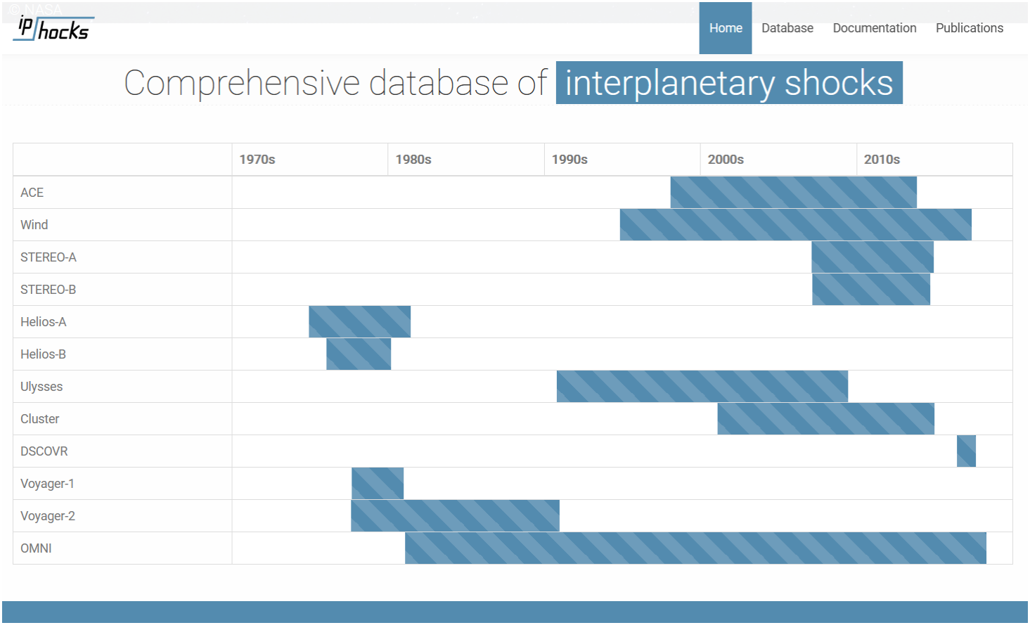
▍4.4 Data acquiring process ▍

There are several steps for the data acquiring process. First of all, to determine the propagation of shocks, shocks that occurred in a single day are needed. For this purpose, shock candidates are chosen from the shock lists in the Database of Heliospheric Shock Waves maintained at the University of Helsinki http://www.ipshocks.fi/ as shown in Figure 4.9.

4.4 数据获取流程

数据获取流程包含以下几个步骤：首先，为确定激波传播特性，需要获取单日内发生的激波事件。为此，从赫尔辛基大学维护的日球层激波数据库中的激波列表中筛选候选激波，详见http://www.ipshocks.fi/（如图4.9所示）。

Figure 4.9: Identified shocks detected by the spacecraft in the list

For the event selection I chose the year 2007 for the reason that STEREO−A and STEREO−B were closer to each other as well as to the Sun-Earth line. Hence, the two events are from this year, particularly on May 07, 2007, and April 23, 2007. In the first event, May 07, 2007, the selected spacecraft are STEREO−A, STEREO−B, Wind, and the four cluster satellites: Cluster-1 (C1), Cluster-2 (C2), Cluster-3 (C3), and Cluster-4 (C4), while for the second event, April 23, 2007, the spacecraft are STEREO−A and B, ACE, and Wind. After choosing the shock candidates, I downloaded the shock data from NASA's Coordinated Data Analysis Web (CDAWeb) https://cdaweb.gsfc.nasa.gov/.

在事件选择中，选择了2007年，原因是STEREO−A和STEREO−B彼此之间以及它们与日地线的距离较近。因此，选取的两个事件均来自该年份，具体为2007年5月7日和2007年4月23日。在第一个事件（2007年5月7日）中，选用的航天器包括STEREO−A、STEREO−B、Wind以及四颗Cluster卫星：Cluster-1（C1）、Cluster-2（C2）、Cluster-3（C3）和Cluster-4（C4）；而在第二个事件（2007年4月23日）中，使用的航天器为STEREO−A和B、ACE以及Wind。选定激波候选事件后，我从NASA的协调数据分析网站（CDAWeb）（https://cdaweb.gsfc.nasa.gov/）下载了激波数据。

I obtained the STEREO− B magnetic field observation and the plasma data from the STEREO In-situ Measurements of Particles and CME Transients magnetic field experiment (IMPACT) (Luhmann et al., 2008) with the time resolution of 100 ms and the STEREO PLAsma and SupraThermal Ion Composition (PLASTIC) (Galvin et al., 2008) respectively. The magnetic field and the plasma data of the STEREO−A and B are in the RTN coordinate system.

获取了STEREO−B的磁场观测数据和等离子体数据，分别来自STEREO原位粒子与CME瞬变磁场实验（IMPACT）（Luhmann et al., 2008），其时间分辨率为100毫秒，以及STEREO等离子体与超热离子成分探测仪（PLASTIC）（Galvin et al., 2008）。STEREO−A和B的磁场和等离子体数据均基于RTN坐标系。

I obtained the Wind magnetic and plasma data from the Magnetic Field Investigation instrument (MFI) (Lepping et al., 1995) with a time resolution of 3 sec and The Solar Wind Experiment (SWE) (Ogilvie et al., 1995) with a time resolution of 1 min respectively. The magnetic field and the plasma data of the Wind are in the Geocentric Solar Ecliptic System (GSE) coordinate system.

获取了Wind卫星的磁场和等离子体数据，分别来自磁场探测仪器（MFI）（Lepping et al., 1995），其时间分辨率为3秒，以及太阳风实验（SWE）（Ogilvie et al., 1995），其时间分辨率为1分钟。Wind卫星的磁场和等离子体数据均基于地心太阳黄道坐标系（GSE）。

I obtained the ACE magnetic and plasma data from the ACE Magnetic Field Experiment (MAG) (Smith et al., 1998) with a time resolution of 1 sec and the Solar Wind Electron Proton Alpha Monitor (SWEPAM) (McComas et al., 1998) with the time resolution of 64 sec, respectively. The magnetic field and the plasma data are in both the RTN and GSE coordinate systems.

获取了ACE卫星的磁场和等离子体数据，分别来自ACE磁场实验（MAG）（Smith et al., 1998），其时间分辨率为1秒，以及太阳风电子质子α粒子监测仪（SWEPAM）（McComas et al., 1998），其时间分辨率为64秒。ACE卫星的磁场和等离子体数据同时采用RTN和GSE坐标系。

I acquired the magnetic data of Cluster satellites from the Cluster Fluxgate Magnetometer (FGM) (Balogh et al., 1997) with a time resolution of 4 sec for all the four Cluster satellites, ion data from the Cluster Ion Spectrometry (CIS) (Reme et al., 1997) with a time resolution of 4 sec for the Cluster-1 and Cluster-3 satellites, and the spacecraft potential data from Electric Fields and Waves (EFW) (Gustafsson et al., 1997) with a time resolution of 4 sec for the Cluster-2 and Cluster-4 satellites. All the Cluster data were in the GSE coordinate system.

获取了Cluster卫星的磁场数据，来自Cluster磁通门磁力计（FGM）（Balogh et al., 1997），其时间分辨率为4秒（适用于所有四颗Cluster卫星）；离子数据来自Cluster离子光谱仪（CIS）（Reme et al., 1997），其时间分辨率为4秒（仅适用于Cluster-1和Cluster-3卫星）；航天器电位数据来自电场与波动探测仪（EFW）（Gustafsson et al., 1997），其时间分辨率为4秒（仅适用于Cluster-2和Cluster-4卫星）。所有Cluster数据均基于GSE坐标系。

2 It is the spacecraft coordinate system and R is radially outward from the Sun, T is along the planetary orbital, and N is northward direction

3 X-axis is pointing to the Sun from the Earth, Y-axis is in the ecliptic plane against the planetary motion and Z-axis is northward direction

4 In which the X-axis is toward the Earth from the Sun, Z-axis is northward direction. This system is fixed with respect to the Sun-Earth line

2 这是航天器坐标系，其中R表示从太阳沿径向向外，T沿行星轨道方向，N为北向。

3 X轴从地球指向太阳，Y轴位于黄道面内且与行星运动方向相反，Z轴为北向。

4 在该系统中，X轴从太阳指向地球，Z轴为北向。此坐标系相对于日地线固定。

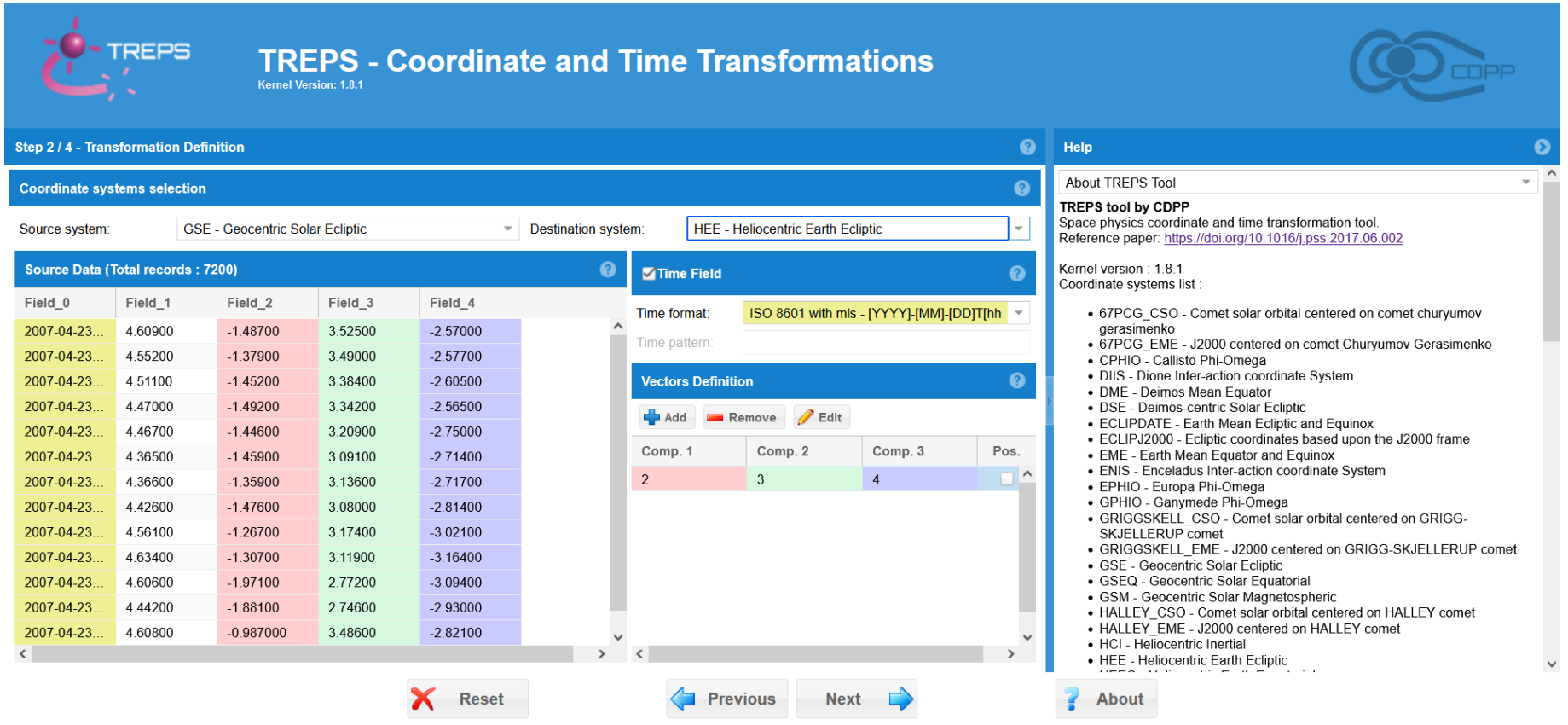
Figure 4.10: TREPS interface, showing a transformation from the GSE to the HEE coordinate system. The green colored column denotes the time field and the other three colored columns denote X, Y, and Z vector components