


Python数据可视化之高斯分布
一维高斯分布模型
高斯分布:
N(μ,δ2)=1δ2π−−√e−(x−μ)22δ2
Python实现
在python中,我们通过坐标变换来求得任意的高斯分布。
import numpy as np
import matplotlib.pyplot as plt

x = np.random.randn(400)
其中np.random.randn(400)生成400个符合正态分布的样本点,背后的生成模型为:
N(0,1)=12π−−√e−x22
可视化数据样本点:
y = np.zeros((400))

plt.plot(x,y,'ro')
plt.axis([-5,5,-0.1,0.2])
plt.show()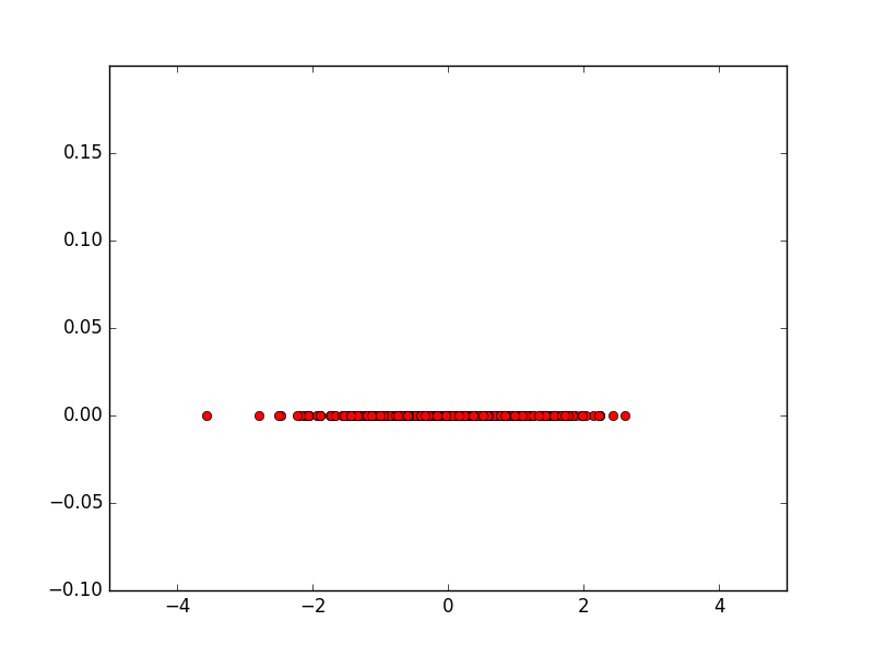
可视化概率分布函数:
n, bins, patches = plt.hist(x, 50, normed=1, facecolor='r', alpha=0.75)
plt.axis([-5,5,0,1])
plt.show()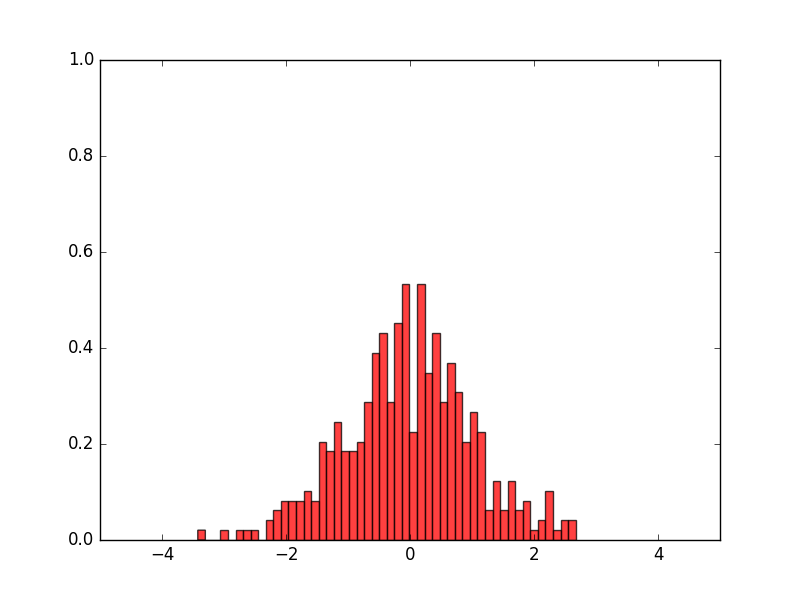
当增大数据样本点时,上述样本分布近似于高斯分布:
x = np.random.randn(100000)
n, bins, patches = plt.hist(x, 50, normed=1, facecolor='r', alpha=0.75)
plt.axis([-5,5,0,1])
plt.show()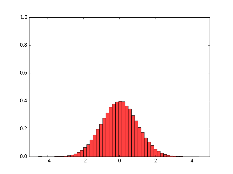
通过坐标变化画出任意高斯分布模型,令
f(x)=12π−−√e−x22
其中np.random.randn()函数生成了大量的x点。所以我们可以让
x=x′−μδ
代入 f(x) 得
f(x′−μδ)=1δ2π−−√e−(x−μ)22δ2
我们不考虑纵轴的变化情况。因此要想得到任意的高斯分布模型,我们只需要解出 x′ 即可,解得 x′=μ+δx
又因为 x <script type="math/tex" id="MathJax-Element-43">x</script>由np.random.randn()生成,所以在python中,我们可以有如下形式:
mu,delta= 70,4.2
x = mu + delta * np.random.randn(100000)
n, bins, patches = plt.hist(x, 50, normed=1, facecolor='r', alpha=0.75)
plt.axis([50,100,0,0.5])
plt.show()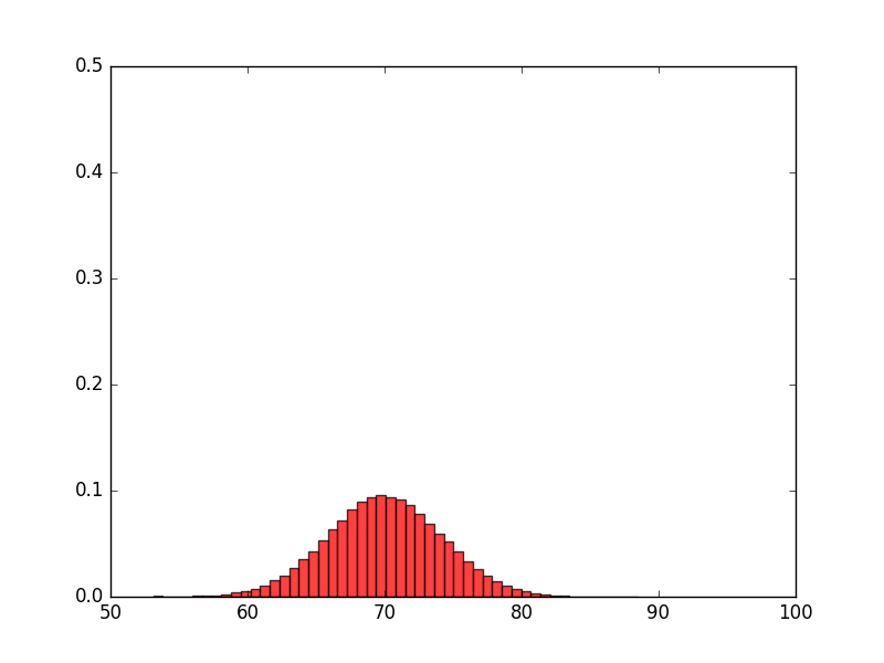
二维高斯分布模型
对应的,只需要生成符合正态分布的x和y即可,代码如下:
mu_x,delta_x= 70,4.2
mu_y,delta_y = 20,2.1
x = mu_x + delta_x * np.random.randn(400)
y = mu_y + delta_y * np.random.randn(400)

plt.plot(x,y,'ro')
plt.axis([50,90,10,30])
plt.show()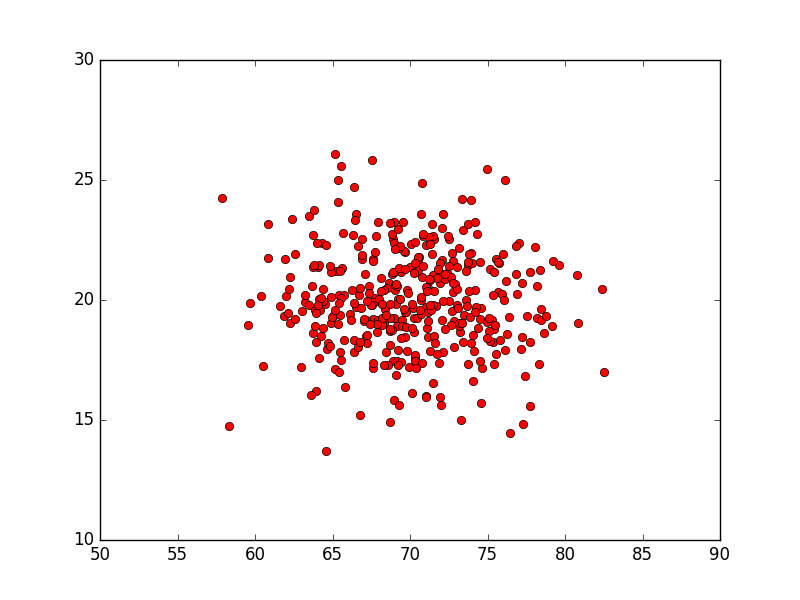


 1607
1607

 被折叠的 条评论
为什么被折叠?
被折叠的 条评论
为什么被折叠?
 到【灌水乐园】发言


