caffe (SGD ADAGRAD NAG BN)

在Deep Learning中，往往loss function是非凸的，没有解析解，我们需要通过优化方法来求解。Caffe通过协调的进行整个网络的前向传播推倒以及后向梯度对参数进行更新，试图减小损失。

 Caffe已经封装好了三种优化方法，分别是Stochastic Gradient Descent (SGD), AdaptiveGradient (ADAGRAD), and Nesterov’s Accelerated Gradient (NAG)。

 Solver的流程：

1.     设计好需要优化的对象，以及用于学习的训练网络和用于评估的测试网络。

2.     通过forward和backward迭代的进行优化来跟新参数

3.     定期的评价测试网络

4.     在优化过程中显示模型和solver的状态

 每一步迭代的过程

1.     通过forward计算网络的输出和loss

2.     通过backward计算网络的梯度

3.     根据solver方法，利用梯度来对参数进行更新

4.     根据learning rate，history和method来更新solver的状态

 

和Caffe模型一样，Caffe solvers也可以CPU / GPU运行。

1. Methods

Solver方法一般用来解决loss函数的最小化问题。对于一个数据集D，需要优化的目标函数是整个数据集中所有数据loss的平均值。

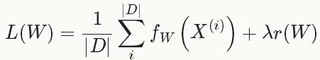
其中， r(W)是正则项，为了减弱过拟合现象。

如果采用这种Loss 函数，迭代一次需要计算整个数据集，在数据集非常大的这情况下，这种方法的效率很低，这个也是我们熟知的梯度下降采用的方法。


在实际中，会采用整个数据集的一个mini-batch，其数量为N<<|D|，此时的loss 函数为：
 


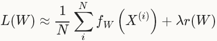
有了loss函数后，就可以迭代的求解loss和梯度来优化这个问题。在神经网络中，用forward pass来求解loss，用backward pass来求解梯度。

1.1 SGD

类型：SGD
随机梯度下降（Stochastic gradient descent）通过negative梯度 和上一次的权重更新值V_t的线性组合来更新W，迭代公式如下：

 
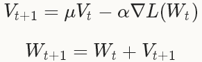
其中，learning rate  是negative梯度的权重，momentum是上一次更行的权重。这两个参数需要通过tuning来得到最好的结果，一般是根据经验设定的。如果你不知道如何设定这些参数，可以参考下面的经验法则，如果需要了解更多的参数设置技巧可以参考论文Stochastic Gradient Descent Tricks [1]。

设置learningrate和momentum的经验法则

例子

[plain]  view plain  copy

1. base_lr: 0.01     # begin training at a learning rate of0.01 = 1e-2  
2.    
3. lr_policy: "step" # learning ratepolicy: drop the learning rate in "steps"  
4.                   # by a factor of gamma everystepsize iterations  
5.    
6. gamma: 0.1        # drop the learning rate by a factor of10  
7.                   # (i.e., multiply it by afactor of gamma = 0.1)  
8.    
9. stepsize: 100000  # drop the learning rate every 100K iterations  
10.    
11. max_iter: 350000  # train for 350K iterations total  
12.    
13. momentum: 0.9  

在深度学习中使用SGD，好的初始化参数的策略是把learning rate设为0.01左右，在训练的过程中，如果loss开始出现稳定水平时，对learning rate乘以一个常数因子（比如，10），这样的过程重复多次。此外，对于momentum，一般设为0.9，momentum可以让使用SGD的深度学习方法更加稳定以及快速，这次初始参数参论文ImageNet Classification with Deep Convolutional Neural Networks [2]。

上面的例子中，初始化learning rate的值为0.01，前100K迭代之后，更新learning rate的值（乘以gamma）得到0.01*0.1=0.001，用于100K-200K的迭代，一次类推，直到达到最大迭代次数350K。

Note that the momentum setting μ effectively multiplies the size of your updates by a factor of 11−μ after many iterations of training, so if you increase μ, it may be a good idea to decrease α accordingly (and vice versa).

For example, with μ=0.9, we have an effective update size multiplier of 11−0.9=10. If we increased the momentum to μ=0.99, we’ve increased our update size multiplier to 100, so we should drop α (base_lr) by a factor of 10.

上面的设置只能作为一种指导，它们不能保证在任何情况下都能得到最佳的结果，有时候这种方法甚至不work。如果学习的时候出现diverge（比如，你一开始就发现非常大或者NaN或者inf的loss值或者输出），此时你需要降低base_lr的值（比如，0.001），然后重新训练，这样的过程重复几次直到你找到可以work的base_lr。

1.2 AdaGrad

类型：ADAGRAD

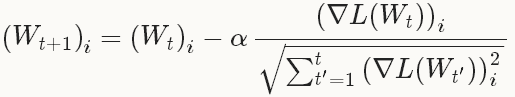
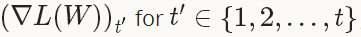
自适应梯度（adaptive gradient）[3]是基于梯度的优化方法（like SGD），以作者的话说就是，“find needles in haystacks in the form of very predictive but rarely seen features”。给定之前所有迭代的更新信息 ，每一个W的第i个成分的更新如下：

 
在实践中需要注意的是，权重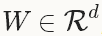，AdaGrad的实现（包括在Caffe中）只需要使用额外的存储来保存历史的梯度信息，而不是的存储（这个需要独立保存每一个历史梯度信息）。（自己没有理解这边的意思）

1.3 NAG

类型：NAG
Nesterov 的加速梯度法（Nesterov’s accelerated gradient）作为凸优化中最理想的方法，其收敛速度可以达到 而不是 。但由于深度学习中的优化问题往往是非平滑的以及非凸的（non-smoothness and non-convexity），在实践中NAG对于某类深度学习的结构可以成为非常有效的优化方法，比如deep MNIST autoencoders[5]。


权重的更新和SGD的的非常类似：

 
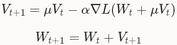
不同的是在计算梯度的时候，在NAG中求解权重加上momentum的梯度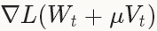，而在SGD中只是简单的计算当前权重的梯度。

一：BN的解释：

在训练深层神经网络的过程中, 由于输入层的参数在不停的变化, 因此, 导致了当前层的分布在不停的变化, 这就导致了在训练的过程中, 要求 learning rate 要设置的非常小, 另外, 对参数的初始化的要求也很高. 作者把这种现象称为 internal convariate shift . Batch Normalization 的提出就是为了解决这个问题的. BN 在每一个 training mini-batch 中对每一个 feature 进行 normalize. 通过这种方法, 使得网络可以使用较大的 learning rate, 而且, BN 具有一定的 regularization 作用.

（BN在知乎上的一个解释：

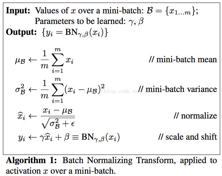
顾名思义，batch normalization嘛，就是“ 批规范化”咯。Google在ICML文中描述的非常清晰，即在每次SGD时，通过mini-batch来对相应的activation做规范化操作，使得结果（输出信号各个维度）的均值为0，方差为1. 而最后的“scale and shift”操作则是为了让因训练所需而“刻意”加入的BN能够有可能还原最初的输入（即当

），从而保证整个network的capacity。（有关capacity的解释：实际上BN可以看作是在原模型上加入的“新操作”，这个新操作很大可能会改变某层原来的输入。当然也可能不改变，不改变的时候就是“还原原来输入”。如此一来，既可以改变同时也可以保持原输入，那么模型的容纳能力（capacity）就提升了。）以上部分的链接：https://www.zhihu.com/question/38102762/answer/85238569

）

Batch Normalization 算法

二：caffe中的batch_norm层

Reshape()中是bn层需要的一些变量的初始化，代码如下

[cpp]  view plain  copy

 

1. template <typename Dtype>  
2. void BatchNormLayer<Dtype>::Reshape(const vector<Blob<Dtype>*>& bottom,  
3.       const vector<Blob<Dtype>*>& top) {  
4.   if (bottom[0]->num_axes() >= 1)  
5.     CHECK_EQ(bottom[0]->shape(1), channels_);  
6.   top[0]->ReshapeLike(*bottom[0]);  
7.   
8.   vector<int> sz;  
9.   sz.push_back(channels_);  
10.   mean_.Reshape(sz);//通道数,即channel值大小，存储的是均值  
11.   variance_.Reshape(sz);//通道数，即channel值大小，存储的是方差值  
12.   temp_.ReshapeLike(*bottom[0]);//temp_中存储的是减去mean_后的每一个数的方差值。  
13.   x_norm_.ReshapeLike(*bottom[0]);  
14.   sz[0]=bottom[0]->shape(0);  
15.   batch_sum_multiplier_.Reshape(sz);//batch_size 大小  
16.   
17.   int spatial_dim = bottom[0]->count()/(channels_*bottom[0]->shape(0));//图像height*width  
18.   
19.   /* 
20.   *spatial_sum_multiplier_是一副图像大小的空间(height*width)，并初始化值为 1 ， 
21.   *作用是在计算mean_时辅助通过乘的方式将一副图像的值相加，结果是一个数值 
22.   */  
23.   if (spatial_sum_multiplier_.num_axes() == 0 ||  
24.       spatial_sum_multiplier_.shape(0) != spatial_dim) {  
25.     sz[0] = spatial_dim;  
26.     spatial_sum_multiplier_.Reshape(sz);  
27.     Dtype* multiplier_data = spatial_sum_multiplier_.mutable_cpu_data();//分配一副图像的空间  
28.     caffe_set(spatial_sum_multiplier_.count(), Dtype(1), multiplier_data);//初始化值为 1，   
29.   }  
30.   
31.   int numbychans = channels_*bottom[0]->shape(0);//batch_size*channel  
32.   if (num_by_chans_.num_axes() == 0 ||  
33.       num_by_chans_.shape(0) != numbychans) {  
34.     sz[0] = numbychans;  
35.     num_by_chans_.Reshape(sz);  
36.   
37.     //batch_sum_multiplier_ batch_size大小的空间，也是辅助在计算mean_时，将所要图像的相应的通道值相加。  
38.     caffe_set(batch_sum_multiplier_.count(), Dtype(1),  
39.         batch_sum_multiplier_.mutable_cpu_data());//分配空间，初始化为 1，  
40.   }  
41. }  

Forwad_cpu()函数中，计算均值和方差的方式，都是通过矩阵-向量乘的方式来计算。计算过程，对照上面的公式，代码如下：

[cpp]  view plain  copy

 

1. template <typename Dtype>  
2. void BatchNormLayer<Dtype>::Forward_cpu(const vector<Blob<Dtype>*>& bottom,  
3.     const vector<Blob<Dtype>*>& top) {  
4.   const Dtype* bottom_data = bottom[0]->cpu_data();  
5.   Dtype* top_data = top[0]->mutable_cpu_data();  
6.   int num = bottom[0]->shape(0);  
7.   int spatial_dim = bottom[0]->count()/(bottom[0]->shape(0)*channels_);//spatial_dim值是 图像height*width  
8.   
9. //如果底层的blob与顶层的blob不是同一个blob  
10.   if (bottom[0] != top[0]) {  
11.     caffe_copy(bottom[0]->count(), bottom_data, top_data);  
12.   }  
13.   
14.   if (use_global_stats_) {  
15.     // use the stored mean/variance estimates.  
16.     const Dtype scale_factor = this->blobs_[2]->cpu_data()[0] == 0 ?  
17.         0 : 1 / this->blobs_[2]->cpu_data()[0];  
18.     caffe_cpu_scale(variance_.count(), scale_factor,  
19.         this->blobs_[0]->cpu_data(), mean_.mutable_cpu_data());  
20.     caffe_cpu_scale(variance_.count(), scale_factor,  
21.         this->blobs_[1]->cpu_data(), variance_.mutable_cpu_data());  
22.   } else {  
23.     // compute mean 计算均值  
24.     //将每一副图像值相加为一个值，共有channels_ * num个值，然后再乘以 1/num*spatial_dim，结果存储到blob num_by_chans_中  
25.     caffe_cpu_gemv<Dtype>(CblasNoTrans, channels_ * num, spatial_dim, //channel*num 行；spatial_dim 列，大小是height*width  
26.         1. / (num * spatial_dim), bottom_data,  
27.         spatial_sum_multiplier_.cpu_data(), 0.,  
28.         num_by_chans_.mutable_cpu_data());  
29.   
30.  //上面计算得到的值大小是num*channel， 将图像的每个通道的值相加，最后获得channel个数值，结果存储到mean_中  
31.     caffe_cpu_gemv<Dtype>(CblasTrans, num, channels_, 1.,  
32.         num_by_chans_.cpu_data(), batch_sum_multiplier_.cpu_data(), 0.,  
33.         mean_.mutable_cpu_data());  
34.   }  
35.   
36.   // subtract mean  
37.   //将channels_个值的均值mean_矩阵扩展到num_*channels_*height*width，并用top_data数据减去均值  
38.   caffe_cpu_gemm<Dtype>(CblasNoTrans, CblasNoTrans, num, channels_, 1, 1,  
39.       batch_sum_multiplier_.cpu_data(), mean_.cpu_data(), 0.,  
40.       num_by_chans_.mutable_cpu_data());  
41.     
42.   caffe_cpu_gemm<Dtype>(CblasNoTrans, CblasNoTrans, channels_ * num,  
43.       spatial_dim, 1, -1, num_by_chans_.cpu_data(),  
44.       spatial_sum_multiplier_.cpu_data(), 1., top_data);//用blob top_data中的数据减去mean_值  
45.   
46.   if (!use_global_stats_) {  
47.     // compute variance using var(X) = E((X-EX)^2)  
48.     caffe_powx(top[0]->count(), top_data, Dtype(2),  
49.         temp_.mutable_cpu_data());  // (X-EX)^2 //对向量的每一个值求方差，结果存储到blob temp_中  
50.     caffe_cpu_gemv<Dtype>(CblasNoTrans, channels_ * num, spatial_dim,  
51.         1. / (num * spatial_dim), temp_.cpu_data(),  
52.         spatial_sum_multiplier_.cpu_data(), 0.,  
53.         num_by_chans_.mutable_cpu_data());//同上计算 mean_的方式，矩阵 向量 乘  
54.     caffe_cpu_gemv<Dtype>(CblasTrans, num, channels_, 1.,  
55.         num_by_chans_.cpu_data(), batch_sum_multiplier_.cpu_data(), 0.,  
56.         variance_.mutable_cpu_data());  // E((X_EX)^2)//同上计算 mean_的方式，矩阵 向量 乘 (此处num_by_chans_转置)  
57.   
58.     // compute and save moving average  
59.     this->blobs_[2]->mutable_cpu_data()[0] *= moving_average_fraction_;  
60.     this->blobs_[2]->mutable_cpu_data()[0] += 1;  
61.   
62.     // blob_[0] = mean_ + moving_average_fraction_* blob_[0];   
63.     caffe_cpu_axpby(mean_.count(), Dtype(1), mean_.cpu_data(),  
64.         moving_average_fraction_, this->blobs_[0]->mutable_cpu_data());//Y=alpha*X+beta*Y;  
65.           
66.     int m = bottom[0]->count()/channels_;// m = num*height*width;  
67.   
68.     //blob_[1] = bias_correction_factor * variance_ + moving_average_fraction_ * blob_[1]  
69.     Dtype bias_correction_factor = m > 1 ? Dtype(m)/(m-1) : 1;  
70.     caffe_cpu_axpby(variance_.count(), bias_correction_factor,  
71.         variance_.cpu_data(), moving_average_fraction_,  
72.         this->blobs_[1]->mutable_cpu_data());  
73.   }  
74.   
75.   // normalize variance  
76.   caffe_add_scalar(variance_.count(), eps_, variance_.mutable_cpu_data());//将 variance 每个值加一个很小的值 eps_,防止除 0的情况。  
77.   caffe_powx(variance_.count(), variance_.cpu_data(), Dtype(0.5),  
78.              variance_.mutable_cpu_data()); // 对 variance的每个值 求开方。  
79.   
80.   // replicate variance to input size  
81.   //以下这两个函数同上面的mean_一样，将channels_个值的方差variance_矩阵扩展到num_*channels_*height*width  
82.   caffe_cpu_gemm<Dtype>(CblasNoTrans, CblasNoTrans, num, channels_, 1, 1,  
83.       batch_sum_multiplier_.cpu_data(), variance_.cpu_data(), 0.,  
84.       num_by_chans_.mutable_cpu_data());  
85.   caffe_cpu_gemm<Dtype>(CblasNoTrans, CblasNoTrans, channels_ * num,  
86.       spatial_dim, 1, 1., num_by_chans_.cpu_data(),  
87.       spatial_sum_multiplier_.cpu_data(), 0., temp_.mutable_cpu_data());  
88.     
89.   caffe_div(temp_.count(), top_data, temp_.cpu_data(), top_data);//top_data 除以 temp_  
90.   // TODO(cdoersch): The caching is only needed because later in-place layers  
91.   //                 might clobber the data.  Can we skip this if they won't?  
92.   caffe_copy(x_norm_.count(), top_data,  
93.       x_norm_.mutable_cpu_data());//将 最后的结果top_data 数据复制 到 x_norm_中。  
94. }  

（完）

2. 参考：

[1] L. Bottou. Stochastic Gradient Descent Tricks. Neural Networks: Tricks of the Trade: Springer, 2012.
[2] A. Krizhevsky, I. Sutskever, and G. Hinton. ImageNet Classification with Deep Convolutional Neural Networks. Advances in Neural Information Processing Systems, 2012.
[3] J. Duchi, E. Hazan, and Y. Singer. Adaptive Subgradient Methods for Online Learning and Stochastic Optimization. The Journal of Machine Learning Research, 2011.
[4] Y. Nesterov. A Method of Solving a Convex Programming Problem with Convergence Rate O(1/k√). Soviet Mathematics Doklady, 1983.
[5] I. Sutskever, J. Martens, G. Dahl, and G. Hinton. On the Importance of Initialization and Momentum in Deep Learning. Proceedings of the 30th International Conference on Machine Learning, 2013.
[6] http://caffe.berkeleyvision.org/tutorial/solver.html