用 Matlab 计算并画出大量数据的CDF

   这篇 blog 将展示用 matlab 计算并画出大量数据的 CDF （累计分布函数）的两种方法。第一种是我自己于2012年写的，后来用的过程中发现有缺陷；后来2014年写另一篇paper时，搜寻到第二种简易又高效的方法。这里我给出它们各自的用例，包括画图用的数据与脚本，以及效果图。For your reference.

============================================================================================

     Section A. 第一种方法

     今天(2012-10-17)有一些数据需要处理，这些数据好不容易从文件中剥离了出来，然后自己写了一个function，计算并控制 plot 这些数据的 CDF 图。因为第一种方法用到的例子的数据文件太大，就没有贴上来。如果有想亲自试验一下这个过程的同学，请参照下文中第二个方法中的完整用例。

% ----------------------- 自实现 CDF 计算 function:  funcCDF.m

[plain] view plaincopy

1. % para@1: CNT_pnts, the number of points to denote the CDF;  
2. % para@2: Range_low, the lower bound of variable;  
3. % para@3: Range_up, the upper bound of variable;  
4. % para@4 : arr_Vals, array of the values to be processed.  
5.   
6. function [x, CDF_Vals] = funcCDF(CNT_pnts, Range_low, Range_up, arr_Vals)  
7. data = sort( arr_Vals' ); % T', horizon arrays of T.  
8. N = length(data);  
9. stepLen = (Range_up-Range_low)/CNT_pnts;  
10. Counter = zeros(1,CNT_pnts);  
11. for i = 1:1:N  
12.     for j = 1:1:CNT_pnts  
13.         if ( data(1,i) <= (Range_low + j*stepLen) )  
14.             Counter(1,j) = Counter(1,j) + 1;  
15.         end  
16.     end  
17. end  
18. CDF = Counter(1,:)./N;  
19. CDF_Vals = CDF(1,:)';  
20. x = (Range_low+stepLen):stepLen:Range_up;  
21. % ---- end of func.  

% --------------------- 2 use cases：

[plain] view plaincopy

1. CNT_pnts = 100;  
2. deadline_N500r1 = 550;  
3. deadline_N500r3 = 270;  
4. deadline_N500r5 = 240;  
5. PntVal_N500Tau100r1 = textread('N500Tau100r1.tr','%*s %*s %*s %*s %*s %*s %*s %*s %*s %*s %*s %.2f');  
6. [x_r1,cdf_r1] = funcCDF(CNT_pnts, 0, deadline_N500r1, PntVal_N500Tau100r1);  
7. plot(x_r1, cdf_r1, 'ob')  
8. hold on  
9.   
10. PntVal_N500Tau100r3 = textread('N500Tau100r3.tr','%*s %*s %*s %*s %*s %*s %*s %*s %*s %*s %*s %.2f');  
11. [x_r3,cdf_r3] = funcCDF(CNT_pnts, 0, deadline_N500r3, PntVal_N500Tau100r3);  
12. plot(x_r3, cdf_r3, 'or')  
13. hold on  
14.   
15. PntVal_N500Tau100r5 = textread('N500Tau100r5.tr','%*s %*s %*s %*s %*s %*s %*s %*s %*s %*s %*s %.2f');  
16. [x_r5,cdf_r5] = funcCDF(CNT_pnts, 0, deadline_N500r5, PntVal_N500Tau100r5);  
17. plot(x_r5, cdf_r5, 'oc')  
18. grid  

% --------------------- 3 效果图：

Fig.1 CDF_N200r3--Tau-60-80-100-100Pnts

Fig.2 CDF_N500Tau100--r-1-3-5-100Pnts

      当把参数 CNT_pnts = 100; 调为 CNT_pnts = 50; 后，显示在图中的点就会减少一半，shows as follow:

Fig.3 CDF_N500Tau100--r-1-3-5-50Pnts

Davy_H （2012-10-17）

============================================================================================

    Section B. 第二种方法

    今天(2014-10-15) 回过头来看这篇blog，前边贴的图太丑，而且其实第一种方法有不完美的地方，即数据少的时候，曲线有时不会从原点开始画。后来寻到更好的方法来画 CDF 图，为了对得起2000+的访问量，所以，今日我决定花些时间，把更好的例子分享出来。

    废话不多说：1）效果图；2）部分数据文件；3）画图的脚本。

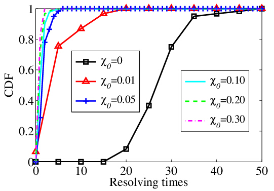
1) ------------------ 

3) ------------------ Codes:

[python] view plaincopy

1. clear;  
2.   
3. % --------------- A. Read the Data.  
4. X_ = textread('_Trace_file.tr','%*s%*s %*s%*s %*s%*s %*s%*s %*s%*s %*s%*s %*s%*s %*s%*s %*s%f');  
5. CNT_resolve_times = textread('_Trace_file.tr','%*s%*s %*s%*s %*s%*s %*s%*s %*s%*s %*s%*s %*s%*s %*s%d %*s%*s' );  
6.   
7.   
8. % --------------- B. Count the the Costs.  
9.   
10. % --------- X_items is the "-Threshold"  
11. X_items =[0.0,0.01,0.05,0.1,0.2,0.3];  
12.   
13. CNT_X = length(X_items);  
14.   
15. % --------- Define the range_x of the x_coordinate in the figure.  
16. step = 1;  
17. range_end = 50;  
18. range_x = 0:step:range_end;  
19.   
20. figure  
21.     % ---------- Format of figure:  
22.     TextFontSize=18;  
23.     LegendFontSize = 16;  
24.     set(0,'DefaultAxesFontName','Times',...  
25.         'DefaultLineLineWidth',2,...  
26.         'DefaultLineMarkerSize',8);  
27.     set(gca,'FontName','Times New Roman','FontSize',TextFontSize);  
28.     set(gcf,'Units','inches','Position',[0 0 6.0 4.0]);  
29.     % ---------- Format of figure:~   
30.       
31.   
32. % ------ Plot lines  
33. for i = 1:1:CNT_X  
34.     Val_item = X_items(i);    
35.     idx_it_Lazy = find( X_ == Val_item );  
36.   
37.     % --- 1 CNT_STimes  
38.     CNT_Re_times_its = [];  
39.     CNT_Re_times_its = CNT_resolve_times( idx_it_Lazy );  
40.       
41.     % --- 2 Plot CDF of CNT_Resloving_times, i.e., the "CNT_STimes" in the trace file.  
42.     if (i==1) linePoint_type = '-sk'; step = 5; range_x = 0:step:range_end;  
43.     elseif (i==2) linePoint_type = '-^r';  
44.     elseif (i==3) linePoint_type = '-+b'; step = 1; range_x = 0:step:range_end;  
45.     elseif (i==4) linePoint_type = '-c';  step = 1; range_x = 0:step:range_end;  
46.     elseif (i==5) linePoint_type = '--g'; step = 1; range_x = 0:step:range_end;  
47.     elseif (i==6) linePoint_type = '-.m'; step = 1; range_x = 0:step:range_end;  
48.     end  
49.       
50.     %%% ====== Critical Code of CDF-Ploting :  
51.     h_rtl = hist( CNT_Re_times_its, range_x );  
52.     pr_approx_cdf = cumsum(h_rtl) / ( sum(h_rtl) );  
53.     %%% ====== Critical Code of CDF-Ploting :~  
54.       
55.     handler = plot( range_x, pr_approx_cdf, linePoint_type );  
56.     if      (i==4) h4 = handler;  
57.     elseif  (i==5) h5 = handler;  
58.     elseif  (i==6) h6 = handler;  
59.     end  
60.     hold on  
61. end  
62.   
63. % --------- Set the other formats of the figure :  
64.     grid off  
65.     axis([0 range_end 0 1.0])  
66.     ylabel('CDF')  
67.     xlabel('Resolving times')  
68.       
69.     % --------- Plot the multi-legends :  
70.     hg1=legend('{\it \chi_0}=0', '{\it \chi_0}=0.01', '{\it \chi_0}=0.05',  0);  
71.     set(hg1,'FontSize',LegendFontSize);  
72.   
73.     ah1 = axes('position',get(gca,'position'), 'visible','off');    
74.   
75.     hg2 = legend(ah1, [h4,h5,h6],  '{\it \chi_0}=0.10','{\it \chi_0}=0.20','{\it \chi_0}=0.30',  0);  
76.     set(hg2,'FontSize',LegendFontSize);  
77.     % --------- Plot the multi-legends :~  
78. % --------- Set the other formats of the figure :~  

    关键代码处，我已经做了注释，此处再强调一下：

    1. 画 CDF 的2句关键代码，其中的3个 functions 请自己查询。

    %%% ====== Critical operation of CDF-Ploting :
    h_rtl = hist ( CNT_Re_times_its, range_x );
    pr_approx_cdf = cumsum(h_rtl) / ( sum(h_rtl) );
    %%% ====== Critical operation of CDF-Ploting :~

  

    2. for 循环中的那一段 if else 语句，是为了设置各条曲线的点线型( linePoint type ) 与 各条线上的取样点的密度。  

    3. 此外，从这个脚本里，也可以额外获取画多个图例 (plot multiple legends) 的方法。

y = evrnd(0,3,100,1);

cdfplot(y);

hold on;

x = -20:0.1:10;

f = evcdf(x,0,3);

plot(x,f,'m');

legend('Empirical','Theoretical','Location','NW')