


# Machine Learning
标签(空格分隔): ML
Introduction
Supervised Learning
Supervised Learning: “right answers” given
Classification: Discrete valued output (0 or 1)
Regression: Predict continuous valued output
Unsupervised Learning
Model and Cost Function
Linear regression with one variable
Univariate linear regression
Hypothesis:
Parameters:
Idea: Choose
θ0,θ1
so that
hθ(x)
is close to
y
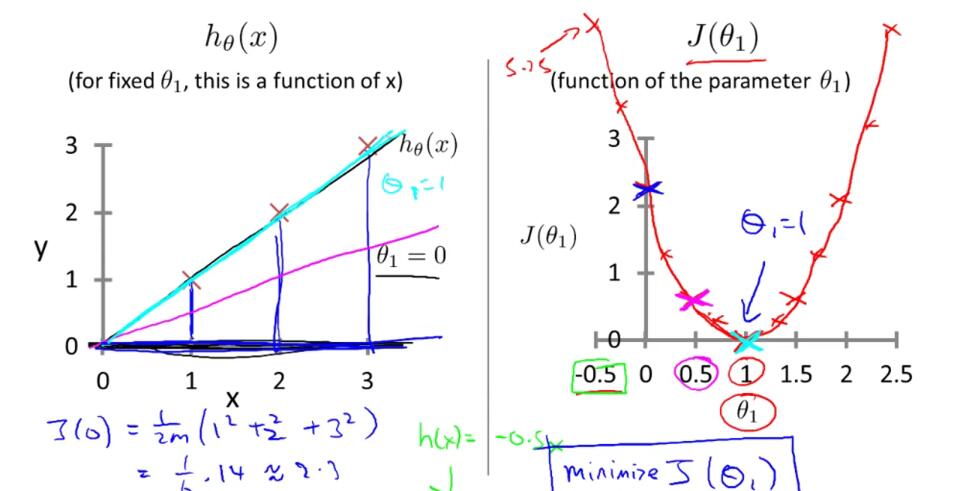
for our training examplesCose Function:
We called that square error function.
hθ(x) (for fixed θ0,θ1 , this is a function of x )
Matrix
Dimension of matrix: number of rows
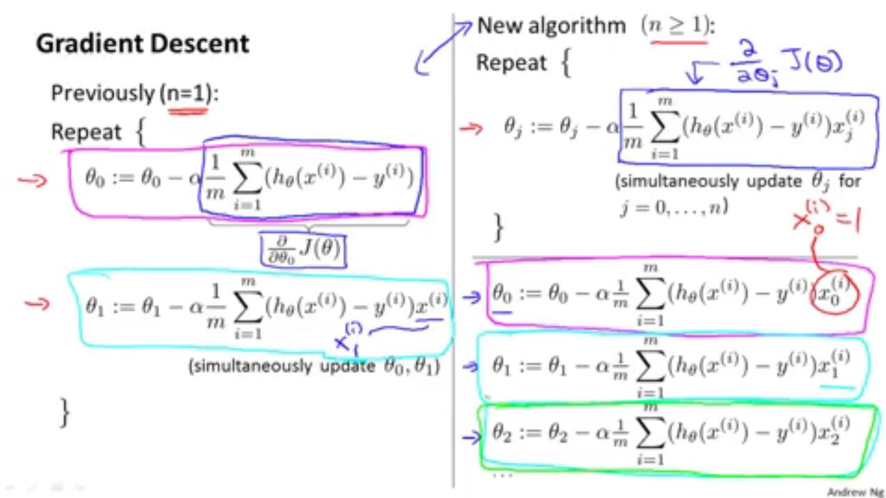
Gradient descent algorithm
repeat until convergence
:= is assignment, and
α
is learning rate.
the subtlety of how you implement gradient descent
Correct: simultaneous update:
temp0:=θ0−α∂J(θ0,θ1)∂θ0
temp1:=θ1−α∂J(θ0,θ1)∂θ1
θ0=temp0
θ1=temp1
Gradient descent can converge to a local minimum, even with the learning rate in a fixed.
As we approach a local minimum, gradient descent will automatically take smaller steps. So, no need to decrease &\alpha$ over time.
WEEK 2
Linear Regression with multiple variables: Multiple Features
x(i)
=input (features) of
i(th)
training example.
xij
=value if feature
j
in
Hypothesis
hθ(x)=θ0+θ1x1+θ2x2+⋯+θnxn
For convenience of notation, define
x0=1
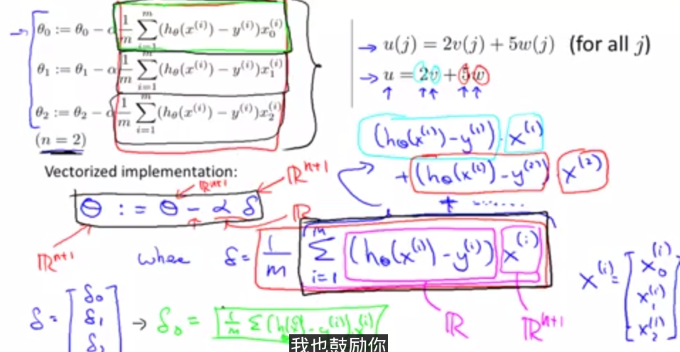
Gradient Descent for Multiple Variables
Hypothesis:
hθ(x)=θT=θ0x0+θ1x1+θ2x2+⋯+θnxn
Parameters:
θ0,θ1,…,θn
Cost function:
Gradient Descent
repeat until convergence
Feature Scaling
Mean Normalization
Learning rate
- “Debugging”: How to make sure gradient descent is working correctly.
- How to choose learning rate α
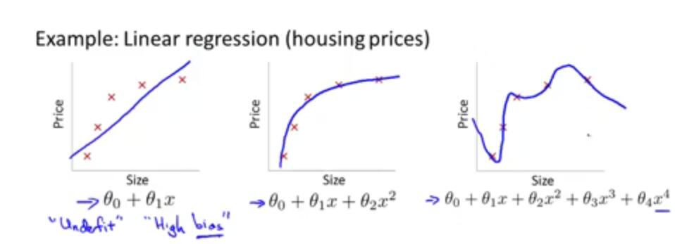
Housing prices prediction
define new features
Polynomial regression
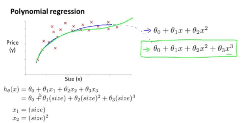
Choice of features
Computing Parameters Analytically
Normal Equation
Method to solve for
θ
analytically.
+ No need to chhose α
+ Don’t need to iterate.
+ Need to compute (XTX)−1
+ Slow if n is very large.
Octave
Moving Data Around
    load('featuresX.dat')
    load featuresX.dat
    who %veriables in the current scope
    whos
    clear
    save hello.mat v
    save hello.txt v %save as text(ASCII)
    A(2,:)  %':' means every elements along that row
    A([1 3],:)
    A = [A,[100;200;300]];
    A[:] %put all elements of A into a single vector
Computing on Data
    A.*B
    A*B
    A.^2
    v=[1;2;3]
    1 ./ v
    log(v)
    exp(v)
    abs(v)
    -v
    v + ones(length(v),1)
    a = [1 2 3 4]
    [val,ind]=max(a)
    a < 1
    find(a<3)
    A = magic(3)
    [r,c] = find(A>=7)
    sum(a)
    prod(a)
    floor(a)
    ceil(a)
    max(rand(3),rand(3))
    max(A,[],1)
    max(A,[],2)
    max(max(A))
    A.*eye(3)
    pinv(A)
Plotting Data
plotVectorization
Week 3
Classification and Represstation
Classification
Logistic Regression:
0≤hθ(x)≤1
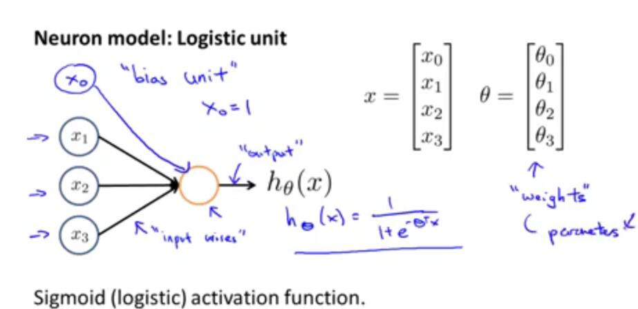
Hypothesis Representation
Logistic Regression Model
want
0≤hθ(x)≤1
Sigmoid function or logistic function
Interpretation of Hypothesis Output
hθ(x)= estimated probability that y=1 on input x
Cost Function
convex
Logistic regression cost function
Note: y=0 or 1 always
Simplified Cost Function
Want minθJ(θ):
Repeat{
(simultaneously update all θj )
}
Algorithm looks identical to linear regression!
Regularization
Overfitting
Cost Function
Gadient descent
Repeat{
}
Non-invertibility (optional/advanced)
Suppose
m≤n,
(#examples) (#features)
if ambda>0,
Week 4
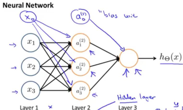
a(j)i=
”activation” of unit i in layer j
Θ(j)=
matrix of weights controlling function mapping from layer j to layer j+1
If network has sj units in layer j ,
Forward propagation: Vectorized implementation


 290
290

 被折叠的 条评论
为什么被折叠?
被折叠的 条评论
为什么被折叠?
 到【灌水乐园】发言


