


Fitting an Orthogonal Regression Using Principal Components Analysis
通过主成分分析进行正交回归拟合
一、背景分析
This example shows how to use Principal Components Analysis (PCA) to fit a linear regression. PCA minimizes the perpendicular distances from the data to the fitted model. This is the linear case of what is known as Orthogonal Regression or Total Least Squares, and is appropriate when there is no natural distinction between predictor and response variables, or when all variables are measured with error. This is in contrast to the usual regression assumption that predictor variables are measured exactly, and only the response variable has an error component.
这个例子展示了如何使用主成分分析(PCA)来进行线性回归拟合。PCA通过最小化数据到拟合模型的垂直距离来实现拟合。这是已知的正交回归或总最小二乘法的线性情况,适用于在自变量和因变量之间没有自然区分,或者当所有变量都受到测量误差的情况。这与通常的回归假设相反,通常回归假设自变量是精确测量的,只有因变量存在误差成分。
For example, given two data vectors x and y, you can fit a line that minimizes the perpendicular distances from each of the points (x(i), y(i)) to the line. More generally, with p observed variables, you can fit an r-dimensional hyperplane in p-dimensional space (r < p). The choice of r is equivalent to choosing the number of components to retain in PCA. It may be based on prediction error, or it may simply be a pragmatic choice to reduce data to a manageable number of dimensions.
举例来说,给定两个数据向量 x 和 y,您可以拟合一条线,最小化每个点 (x(i), y(i)) 到这条线的垂直距离。更一般地,当有 p 个观测变量时,您可以在 p 维空间中拟合一个 r 维超平面(r < p)。选择 r 相当于选择在PCA中要保留的主成分数量。这个选择可以基于预测误差,也可以只是为了将数据降维到一个可管理的维度而做出的实际选择。
In this example, we fit a plane and a line through some data on three observed variables. It's easy to do the same thing for any number of variables, and for any dimension of model, although visualizing a fit in higher dimensions would obviously not be straightforward.
在这个例子中,我们通过一些关于三个观测变量的数据拟合了一个平面和一条直线。同样的方法可以用于任意数量的变量和任意维度的模型,尽管在更高维度中可视化拟合显然不会那么简单。
二、为三维数据拟合平面
Fitting a Plane to 3-D Data
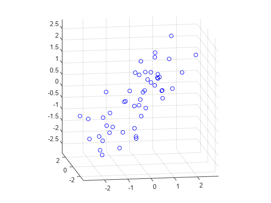
First, we generate some trivariate normal data for the example. Two of the variables are fairly strongly correlated.
首先,我们为这个示例生成一些三元正态分布的数据。其中两个变量之间存在较强的相关性。
rng(5,'twister');
X = mvnrnd([0 0 0], [1 .2 .7; .2 1 0; .7 0 1],50);
plot3(X(:,1),X(:,2),X(:,3),'bo');
grid on;
maxlim = max(abs(X(:)))*1.1;
axis([-maxlim maxlim -maxlim maxlim -maxlim maxlim]);
axis square
view(-9,12);
这段代码用 rng 设定随机种子,方便多次复现同一随机矩阵。mvnrnd 函数设置总体均值为 [0 0 0],并且从正态总体中抽样了 n 个样本,显然这 n 个样本的期望/均值并不一定为 [0 0 0]。随后,将生成的 X 三个特征作为三个坐标轴,利用 plot3 绘制了特征空间。最后对图像进行一些缩放和旋转,使得整体更直观。
知识点:
1.rng 控制随机数生成器
rng用来控制随机种子,一般调用格式为 rng(seed) 或 rng(seed, generator),seed为整型变量,generator则有指定的若干个参数。当使用同一种子时,多次运行代码所产生的随机量相同。另注,若不指定 seed 只指定 generator,需要使用 rng('default') 这种格式。
2.mvnrnd 多元正态随机数
调用格式为 R = mvnrnd(mu, sigma, n) 或 R = mvnrnd(mu, sigma),二者区别简单来看只是生成数据条数(换言之,R的维度)不同,后者只有一行,前者有 n 行。生成的数据矩阵行为不同样本,列为不同特征。该例中均值和协方差矩阵均为 3x3,制定了特征维度为 3,因此生成的 X 大小为 [n, 3]。若用第二种调用格式,则生成数据为 [1, 3]。这里需要注意,sigma 指定的协方差矩阵必须为对称矩阵且半正定。
3.plot3 三维点或线图
plot3 一般调用格式可以描述为 plot3(X1, Y1, Z1, LineSpec1, ..., Xn, Yn, Zn, LineSpecn),其中 i=2~n 这些参数都可以省略。X Y Z 可以为标量、列向量、矩阵,LineSpec 用来指定标记/线型。在本例中,plot3 传入三个 50 维列向量,分别代表 X Y Z 坐标。在绘图时,会按照行的次序画,例如第一个点应当是 (X(1, 1), X(1, 2), X(1, 3)),最后一个点应当是 (X(50, 1), X(50, 2), X(50, 3))。
4.axis 设置坐标轴范围和纵横比
axis(limits) 用于指定坐标轴的范围,需要指定 4、6 或 8 个参数。一般格式为 axis([-X X -Y Y -Z Z])。
axis square 的调用形式为 axis style,用来指定坐标轴尺度。square 使用相同长度的坐标轴线,相应调整数据单位之间的增量。除此之外 style 中还有 tight、normal 等。
5.view 相机视线
为当前坐标区设置相机视线的方位角和仰角。调用格式为 view(az, el),az 为方位角,el 为仰角。
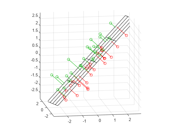
Next, we fit a plane to the data using PCA. The coefficients for the first two principal components define vectors that form a basis for the plane. The third PC is orthogonal to the first two, and its coefficients define the normal vector of the plane.
接下来,我们使用主成分分析(PCA)拟合数据到一个平面。前两个主成分的系数定义了构成平面的基向量。第三个主成分与前两个正交,其系数定义了平面的法向量。
[coeff,score,roots] = pca(X);
basis = coeff(:,1:2)
normal = coeff(:,3)
这段代码使用 pca 函数,三个返回值中包含了所有需要的信息。其中:
1.coeff 主成分系数:指的是 pca 求得的投影矩阵,其是一个方阵,满足 coeff' * coeff = I。其维度和数据特征维度相同。也可以理解成特征矩阵,其中每一列对应一个特征向量。
2.score 主成分得分:指的是原数据点在各成分上的投影坐标。 第一列对应原始数据在第一主成分上的投影值,第二列对应原始数据在第二主成分上的投影值,以此类推。score = X * coeff。
3.roots 特征根/潜在根(也用latent)/特征值:matlab 文档中标准调用格式这里叫 latent,是一个 [1, m] 的矩阵,其中 m 是特征维度。其每个值和 coeff 中的列一一对应,并且以按照从大到小顺序排列。
所以,coeff 的前两列对应前两个主成分的方向向量,而要拟合平面的话这两个方向向量就是平面的基向量。而 pca 的各个主成分相互正交,那么第三主成分就是拟合平面的法向量。
That's all there is to the fit. But let's look closer at the results, and plot the fit along with the data.
就是这样完成了拟合过程。但让我们更仔细地看一下结果,并将拟合结果与数据一起绘制出来。
Because the first two components explain as much of the variance in the data as is possible with two dimensions, the plane is the best 2-D linear approximation to the data. Equivalently, the third component explains the least amount of variation in the data, and it is the error term in the regression. The latent roots (or eigenvalues) from the PCA define the amount of explained variance for each component.
因为前两个主成分解释了数据中尽可能多的方差,所以这个平面是对数据的最佳二维线性近似。等效地说,第三个主成分解释了数据中最少的变异,它是回归中的误差项。PCA 中的潜在根(或特征值)定义了每个主成分所解释的方差量。
pctExplained = roots' ./ sum(roots)pctExplained = 1×3
0.6226 0.2976 0.0798
特征值和方差是有一致性的,特征值大对应主成分所能解释的方差就大(最大可分性),因此可以通过求比例的方法查看各主成分能解释多少方差。在上例中,只有 7% 的方差由第三主成分解释。
The first two coordinates of the principal component scores give the projection of each point onto the plane, in the coordinate system of the plane. To get the coordinates of the fitted points in terms of the original coordinate system, we multiply each PC coefficient vector by the corresponding score, and add back in the mean of the data. The residuals are simply the original data minus the fitted points.
主成分分析的前两个坐标给出了每个数据点在平面上的投影,这是在平面的坐标系中表示的。要获取在原始坐标系中的拟合点的坐标,我们将每个主成分系数向量与相应的分数相乘,然后加回数据的均值。残差就是原始数据减去拟合点。
[n,p] = size(X);
meanX = mean(X,1);
Xfit = repmat(meanX,n,1) + score(:,1:2)*coeff(:,1:2)';
residuals = X - Xfit;
这里的 Xfit 是对 pca 进行重建(恢复)之后的,在原数据空间中的点,并非投影在主成分平面上的点。前面介绍过 score = X * coeff,两侧同乘 coeff' 得到 score * coeff' = X,这是完全恢复,但是此时只取了两个主成分,也就是 score 的前两列乘以系数矩阵的前两列的转置。最后,残差 residual 的值等于原始点减去拟合点。
知识点:
1.mean 数组的均值
mean(A, dim),dim = 1,行压缩,结果是包含每一列均值的行向量;dim = 2,列压缩,结果是包含每一行均值的列向量。
2.repmat 重复数组副本
repmat(A, r1, ...., rn),以本例来说,repmat(meanX, n, 1) 将 meanX 重复 50 行 1 列。目的是为了给拟合点每一行都加上均值(因为前面说过,样本均值不一定等于总体均值)。
The equation of the fitted plane, satisfied by each of the fitted points in Xfit, is ([x1 x2 x3] - meanX)*normal = 0. The plane passes through the point meanX, and its perpendicular distance to the origin is meanX*normal. The perpendicular distance from each point in X to the plane, i.e., the norm of the residuals, is the dot product of each centered point with the normal to the plane. The fitted plane minimizes the sum of the squared errors.
拟合平面的方程 ([x1 x2 x3] - meanX) * normal = 0 适用于Xfit中的每个拟合点。这个平面经过点 meanX,并且它到原点的垂直距离是 meanX * normal。从X中的每个点到平面的垂直距离,即残差的范数,是每个中心化点与平面法向量的点积。拟合平面最小化了平方误差的总和。
error = abs((X - repmat(meanX,n,1))*normal);
sse = sum(error.^2)
sse = 15.5142
X 减去均值是为了中心化,随后乘以平面法向量就可以得到 centeredX 到拟合平面的距离,每个值平方相加后就得到了 sum of squared error - sse。
To visualize the fit, we can plot the plane, the original data, and their projection to the plane.
[xgrid,ygrid] = meshgrid(linspace(min(X(:,1)),max(X(:,1)),5), ...
                         linspace(min(X(:,2)),max(X(:,2)),5));
zgrid = (1/normal(3)) .* (meanX*normal - (xgrid.*normal(1) + ygrid.*normal(2)));
h = mesh(xgrid,ygrid,zgrid,'EdgeColor',[0 0 0],'FaceAlpha',0);

hold on
above = (X-repmat(meanX,n,1))*normal < 0;
below = ~above;
nabove = sum(above);
X1 = [X(above,1) Xfit(above,1) nan*ones(nabove,1)];
X2 = [X(above,2) Xfit(above,2) nan*ones(nabove,1)];
X3 = [X(above,3) Xfit(above,3) nan*ones(nabove,1)];
plot3(X1',X2',X3','-', X(above,1),X(above,2),X(above,3),'o', 'Color',[0 .7 0]);
nbelow = sum(below);
X1 = [X(below,1) Xfit(below,1) nan*ones(nbelow,1)];
X2 = [X(below,2) Xfit(below,2) nan*ones(nbelow,1)];
X3 = [X(below,3) Xfit(below,3) nan*ones(nbelow,1)];
plot3(X1',X2',X3','-', X(below,1),X(below,2),X(below,3),'o', 'Color',[1 0 0]);

hold off
maxlim = max(abs(X(:)))*1.1;
axis([-maxlim maxlim -maxlim maxlim -maxlim maxlim]);
axis square
view(-9,12);
知识点:
1.meshgrid 二维和三维网格
这个函数是用来返回格子坐标的,比如 X = [1, 2, 3], Y = [1, 2, 3],这两个坐标范围就有九个格子,(1, 1), (1, 2), (1, 3), (2, 1), (2, 2), ..., (3, 3),meshgrid 就是干这个事的,两个参数都是个 [1, 5] 的矩阵,返回的结果 xgrid 和 ygrid 都是 [5, 5] 的矩阵,它们的对应位置就是之后要用 mesh 画的网格点,比如 (xgrid(1, 1), ygrid(1, 1)), (xgrid(1, 2), ygrid(1,2)), ..., (xgrid(5,5), ygrid(5,5)),一共 25 个点。
2.linspace 生成线性间距向量
本例中,linspace(min(X(:,1)),max(X(:,1)),5) 是从 X 第一列中最小值到 X 第一列中最大值均分并返回 5 个值。
3.zgrid 的算法
首先平面一般方程为 Ax + By + Cz + D = 0,[A, B, C] 是平面法向量,D 是平面偏移量。写成向量形式,平面法向量是 normal,并且已知 meanX 在拟合平面上,那么就有 normal * meanX + D = 0,可以解出 D。现在 x 和 y 是已知量(保存在 xgrid 和 ygrid)中,求 z 就是解方程。normal(1) * xgrid + normal(2) * ygrid + normal(3) * zgrid - normal * meanX = 0。
4.plot3
这里可以把 plot3(X1',X2',X3','-', X(above,1),X(above,2),X(above,3),'o', 'Color',[0 .7 0]); 拆开看:plot3(X1',X2',X3','-') 和 plot3(X(above,1),X(above,2),X(above,3),'o'),最后设置颜色。第二句比较好理解就是把拟合点用圆圈标出来。第一句,X1 X2 X3 是 [m, 3] 的矩阵(m取决于above 中有多少个 1),转置之后大小是 [3, m],plot3 接收了三个这样的矩阵作为参数,这里其实并不复杂。为了方便理解,其实可以把 nan*ones(nabove,1) 省略掉,这样 X1' X2' X3' 就都是 [2, m] 的矩阵,绘制点的时候,以 X1' X2' X3' 第一行的点为起点,如 (X1'(1, 1), X2'(1, 1), X3'(1, 1)),以 X1' X2' X3' 第二行的点为终点(列和起点要对应),如 (X1'(2, 1), X2'(2, 1), X3'(2, 1)),并且用实线连接两点。更通俗一点,X1' 第一行的点就是起点的 x 坐标,第二行的点就是终点的 x 坐标,X2' 和 X3' 分别对应 y 和 z。nan*ones(nabove,1) 是用来占位的,意义不明。
三、为三维数据拟合直线
Fitting a Line to 3-D Data
Fitting a straight line to the data is even simpler, and because of the nesting property of PCA, we can use the components that have already been computed. The direction vector that defines the line is given by the coefficients for the first principal component. The second and third PCs are orthogonal to the first, and their coefficients define directions that are perpendicular to the line. The simplest equation to describe the line is meanX + t*dirVect, where t parameterizes the position along the line.
将一条直线拟合到数据中甚至更简单,由于PCA的嵌套性质,我们可以使用已经计算的主成分。定义直线的方向向量由第一个主成分的系数给出。第二和第三个主成分与第一个主成分正交,它们的系数定义了与直线垂直的方向。描述这条直线的最简单方程是 meanX + t*dirVect,其中 t 参数化了沿着直线的位置。
dirVect = coeff(:,1)空间直线的一般方程可以描述为:r = r₀ + td,其中 r 是直线上的点的位置矢量,r₀ 是直线上的一点,d 是直线的方向向量,t 是一个参数。meanX 已知在直线上,t 是参数,dirVect 是第一主成分,那么 r = meanX + t * dirVect。
The first coordinate of the principal component scores gives the projection of each point onto the line. As with the 2-D fit, the PC coefficient vectors multiplied by the scores the gives the fitted points in the original coordinate system.
主成分得分的第一个坐标表示每个点在直线上的投影。与二维拟合类似,主成分系数向量乘以得分给出了在原始坐标系中的拟合点。
Xfit1 = repmat(meanX,n,1) + score(:,1)*coeff(:,1)';Plot the line, the original data, and their projection to the line.
绘制这条直线、原始数据以及它们在直线上的投影。
t = [min(score(:,1))-.2, max(score(:,1))+.2];
endpts = [meanX + t(1)*dirVect'; meanX + t(2)*dirVect'];
plot3(endpts(:,1),endpts(:,2),endpts(:,3),'k-');

X1 = [X(:,1) Xfit1(:,1) nan*ones(n,1)];
X2 = [X(:,2) Xfit1(:,2) nan*ones(n,1)];
X3 = [X(:,3) Xfit1(:,3) nan*ones(n,1)];
hold on
plot3(X1',X2',X3','b-', X(:,1),X(:,2),X(:,3),'bo');
hold off
maxlim = max(abs(X(:)))*1.1;
axis([-maxlim maxlim -maxlim maxlim -maxlim maxlim]);
axis square
view(-9,12);
grid on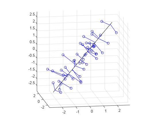


 6651
6651


 被折叠的 条评论
为什么被折叠?
被折叠的 条评论
为什么被折叠?
 到【灌水乐园】发言


