


 本文详细介绍了霍夫变换的基本概念,从直线检测扩展到圆和曲线,解释了参数空间转换过程,并通过MATLAB实例展示了如何在图像处理中使用霍夫变换检测直线、提取峰值和绘制直线段。还探讨了矩形检测的应用和自定义Hough变换的实现。
霍夫变换
霍夫变换是1972年提出来的,最开始就是用来在图像中过检测直线,后来扩展能检测圆、曲线等。
直线的霍夫变换就是 把xy空间的直线 换成成 另一空间的点。就是直线和点的互换。
我们在初中数学中了解到,一条直线可以用如下的方程来表示:y=kx+b,k是直线的斜率,b是截距。
我们转换下变成:b=-kx+y。我们是不是也可以把(k,b)看作另外一个空间中的点?这就是k-b参数空间。 这样,我们就把一条x-y直线用一个(k,b)的点表示出来了。
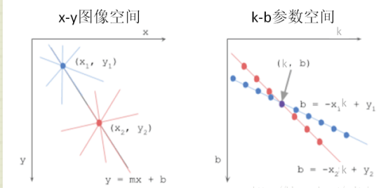
我们看到,在x-y图像空间中的一个点,变成了k-b参数空间中的一条直线,而x-y图像空间中的2点连成的直线,变成了k-b参数空间中的一个交点。
如果x-y图像空间中有很多点在k-b空间中相交于一点,那么这个交点就是我们要检测的直线。这就是霍夫变换检测直线的基本原理。
当然,有一个问题需要注意,图像空间中如果一条直线是垂直的,那么斜率k是没有定义的(或者说无穷大)。为了避免这个问题,霍夫变换采用了另一个参数空间:距离-角度参数空间。也就是极坐标。
我们在中学中学过,平面上的一个点也可以用距离-角度来定义,也就是极坐标。那么在图像中,每一个点都可以用距离和角度来表达:

但是,使用距离-角度后,点(x,y)与距离,角度的关系变成了:
ρ=xcosθ+ysinθ
于是,在新的距离-角度参数空间中,图像中的一个点变成了一个正弦曲线,而不是k-b参数空间中的直线了。这些正弦曲线的交点就是图像空间中我们要检测的直线了。
Matlab霍夫变换的函数详解
[H, theta, rho] = hough(BW,ParameterName, ParameterValue)
BW:二值图
ParameterName:'RhoResolution'或'Theta'
RhoResolution-指定在累计数组中(检测极值)的检测间隔?默认为1
Theta-指定检测的角度范围(不超过-90~90度)以及间隔,例如-90:0.5:89.5,默认-90:1:89
H:累计数组
Theta:H对应的θ,实际上H的大小就是Rho×Theta
Rho:H对应的ρ
这两个参数值的注意,RhoResolution太大覆盖不到极值点,检测到一些不对应直线的次极值,
峰值提取
peaks = houghpeaks(H,numpeaks)
peaks = houghpeaks(...,param1, val1, param2, val2)
H:累计数组;
Numpeaks:指定需要检测的峰值个数;
Param1:可以是'Threshold'或'NHoodSize'
'Threshold'-指定峰值的域值,默认是0.5*max(H(:))
'NHoodSize'-是个二维向量[m,n],检测到一个峰值后,将峰值周围[m,n]内元素置零。
画直线段
lines = houghlines(BW,theta, rho, peaks)
lines = houghlines(...,param1, val1, param2, val2)
BW:二值图
Theta、rho、peaks:分别来自函数hough和houghpeaks
Lines:结构数组,大小等于检测到的直线段数,每个单元包含
Point1、point2:线段的端点
Theta、rho:线段的theta和rho
下面实例演示
用霍夫变换判断矩形
所用图形是我用画图工具制作的,图片很干净,所以不需要滤波等措施。以下是图案。
img = imread('a.png');
img_gray = rgb2gray(img);
%背景是黑的!!!
threshold =graythresh(img_gray);%取阈值
bw=im2bw(img_gray,threshold);
if length(bw(bw==1))>length(bw(bw==0))
bw=~bw;
end
%填充
bw = imfill(bw,'holes');
figure(), imshow(img_gray), title('image');
[B,L] = bwboundaries(bw,'noholes');
stats = regionprops(L,'Area','Centroid','image');
boundary = B{1};
delta_sq = diff(boundary).^2;
perimeter = sum(sqrt(sum(delta_sq,2)));
% obtain the area calculation corresponding
area = stats(1).Area;
% compute the roundness metric
metric = 4*pi*area/perimeter^2;
if metric>0.9
disp('yuan')
else
% the canny edge of image
BW = edge(bw,'canny');
% Iedge=edge(Ihsv,'sobel'); %边沿检测
%BW = imdilate(BW,ones(3));%图像膨胀
figure(), imshow(BW), title('image edge');
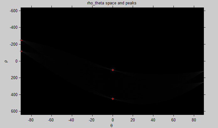
% the theta and rho of transformed space
[H,Theta,Rho] = hough(BW,'RhoResolution',1.2);
figure(), imshow(H,[],'XData',Theta,'YData',Rho,'InitialMagnification','fit'),...
title('rho\_theta space and peaks');
xlabel('\theta'), ylabel('\rho');
axis on, axis normal, hold on;
% label the top 5 intersections
P = houghpeaks(H,4,'threshold',ceil(0.1*max(H(:))),'NHoodSize',[35,11]);
x = Theta(P(:,2));
y = Rho(P(:,1));
plot(x,y,'*','color','r');
% find lines and plot them
lines = houghlines(BW,Theta,Rho,P);
figure(), imshow(img),title('final image');
hold on
b_len = ones(1,length(lines));
for k = 1:length(lines)
xy = [lines(k).point1; lines(k).point2];
b_len(1,k)=sqrt((xy(1,1)-xy(2,1))^2+(xy(1,2)-xy(2,2))^2);
plot(xy(:,1),xy(:,2),'LineWidth',2,'Color','r');
hold on
end
if var(b_len)<10
disp('正方形')
else
disp('长方形')
end
end
然后得到结果
变换参数域图像(很完美,4个点)
结果图像
基本包含在原图形上,测试成功!
参考文献:
[1] http://blog.sina.com.cn/s/blog_ac7218750101giyf.html
[2] https://blog.csdn.net/saltriver/article/details/80547245
[3] https://ww2.mathworks.cn/help/images/ref/hough.html
盘外篇
自己写个Hough变换? hough的原理很简单,可以自己尝试以下。
那么我们检测一下 直线的斜率。
下面上代码
clear all;
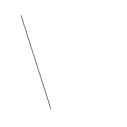
img = imread('demo1.png');
img_gray = rgb2gray(img);
%二值化
threshold =graythresh(img_gray);%取阈值
bw=im2bw(img_gray,threshold);
if length(bw(bw==1))>length(bw(bw==0))
bw=~bw;
end
figure(), imshow(bw), title('image');
% %填充
% bw = imfill(bw,'holes');
% %边沿检测
%the canny edge of image
%bw = edge(bw,'canny');
bw = imdilate(bw,ones(8)); %图像膨胀(因为直线太细会使误差增大)
%figure(), imshow(bw), title('image ');
%the theta and rho of transformed space
[H,Theta,Rho] = hough1(bw);
figure(), imshow(H,[],'XData',Theta,'YData',Rho,'InitialMagnification','fit'),...
title('rho\_theta space and peaks');
xlabel('\theta'), ylabel('\rho');
axis on, axis normal, hold on;
%label the top 1 intersections
%P = houghpeaks(H,1);
[xx,yy]=find(H==max(max(H)),1);
P=[xx,yy];
x = Theta(P(:,2));
y = Rho(P(:,1));
plot(x,y,'*','color','r');
[m,n]=size(bw);
label=zeros(m,n);
xy=[];
for ii=1:length(bw)
jj=ceil((y-ii*cos(x/180*pi))/sin(x/180*pi));
if jj>=1&& jj<=n
label(ii,jj)=1;
if bw(ii,jj)==1
xy=[xy;jj,ii]; %因为plot和imshow的xy轴是镜像关系!
end
end
end
%find lines and plot them
%lines = houghlines(bw,Theta,Rho,P);
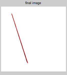
figure(), imshow(img),title('final image');
hold on
plot(xy(:,1),xy(:,2),'LineWidth',2,'Color','r');
k=-sin(x/180*pi)/cos(x/180*pi);
b=y/cos(x/180*pi);
disp(['斜率是',num2str(k)])
disp(['y轴截距是',num2str(b)])
%ezplot('x*cos(-72/180*pi)+y*sin(-72/180*pi)=-31',[0,256])
下面就是自己写的hough变换函数了
function [h, theta, rho] = hough1(f, dtheta, drho)

if  nargin < 3
   drho = 1;
end
if  nargin < 2
   dtheta = 1;
end

f = double(f);
[M,N] = size(f);
theta = linspace(-90, 0, ceil(90/dtheta) + 1);
theta = [theta -fliplr(theta(2:end - 1))];
ntheta = length(theta);

D = sqrt((M - 1)^2 + (N - 1)^2);
q = ceil(D/drho);
nrho = 2*q - 1;
rho = linspace(-q*drho, q*drho, nrho);

[x, y, val] = find(f);
x = x - 1;  y = y - 1;

h = zeros(nrho, length(theta));

for  k = 1:ceil(length(val)/1000)
   first = (k - 1)*1000 + 1;
   last  = min(first+999, length(x));

   x_matrix     = repmat(x(first:last), 1, ntheta);
   y_matrix     = repmat(y(first:last), 1, ntheta);
   val_matrix   = repmat(val(first:last), 1, ntheta);
   theta_matrix = repmat(theta, size(x_matrix, 1), 1)*pi/180;

   rho_matrix = x_matrix.*cos(theta_matrix) + ...
       y_matrix.*sin(theta_matrix);
   slope = (nrho - 1)/(rho(end) - rho(1));
   rho_bin_index = round(slope*(rho_matrix - rho(1)) + 1);

   theta_bin_index = repmat(1:ntheta, size(x_matrix, 1), 1);

   h = h + full(sparse(rho_bin_index(:), theta_bin_index(:), ...
                       val_matrix(:), nrho, ntheta));
end
结果还不错


 被折叠的 条评论
为什么被折叠?
被折叠的 条评论
为什么被折叠?
 到【灌水乐园】发言


