


一、SVM算法
- 支持向量机(Support Vector Machine,常简称为SVM)是一种监督式学习的方法,可广泛地应用于统计分类以及回归分析。
- 它是将向量映射到一个更高维的空间里,在这个空间里建立有一个最大间隔超平面。在分开数据的超平面的两边建有两个互相平行的超平面,分隔超平面使两个平行超平面的距离最大化。假定平行超平面间的距离或差距越大,分类器的总误差越小。
1.核方法
在线性 SVM 中转化为最优化问题时求解的公式计算都是以内积(dot product)形式出现的,其中 ϕ ( X ) \phi(X)ϕ(X ) 是把训练集中的向量点转化到高维的非线性映射函数,因为内积的算法复杂度非常大,所以我们利用核函数来取代计算非线性映射函数的内积。
以下核函数和非线性映射函数的内积等同,但核函数 K 的运算量要远少于求内积。
K ( X i , X j ) = ϕ ( X i ) ⋅ ϕ ( X j ) K(X_i,X_j)=\phi(X_i)·\phi(X_j)K (X i ,X j )=ϕ(X i )⋅ϕ(X j )
(1)常用的核函数
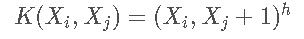
h 度多项式核函数(polynomial kernel of degree h):
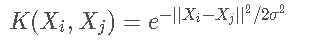
高斯径向基核函数(Gaussian radial basis function kernel):
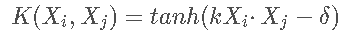
S 型核函数(Sigmoid function kernel):
如何选择使用哪个 kernel ?
- 根据先验知识,比如图像分类,通常使用 RBF(高斯径向基核函数),文字不使用 RBF。
- 尝试不同的 kernel,根据结果准确度而定尝试不同的 kernel,根据结果准确度而定。
(2)核函数举例
假设定义两个向量:
定义方程:

核函数: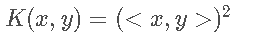
假设: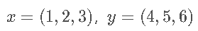
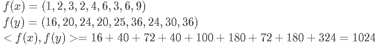
不用核函数,直接求内积:
使用核函数:
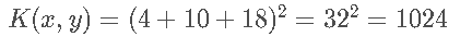
同样的结果,使用 kernel 方法计算容易很多。而这只是 9 维的情况,如果维度更高,那么直接求内积的方法运算复杂度会非常大。
所以使用 kernel 的意义在于:
- 将向量的维度从低维映射到高维
- 降低运算复杂度降低运算复杂度
二、 月亮数据集
x_moom, y_moom = datasets.make_moons()

plt.scatter(x_moom[y_moom==0,0],x_moom[y_moom==0,1])
plt.scatter(x_moom[y_moom==1,0],x_moom[y_moom==1,1])
plt.show()

x_moom, y_moom = datasets.make_moons(noise=0.15,random_state=520)

plt.scatter(x_moom[y_moom==0,0],x_moom[y_moom==0,1])
plt.scatter(x_moom[y_moom==1,0],x_moom[y_moom==1,1])
plt.show()

- 多项式拟合
poly_svc_moom = PolynomialSVC(degree=5,C=10)

poly_svc_moom.fit(x_moom,y_moom)

print("权重w:",poly_svc_moom.named_steps['linearSVC'].coef_[0])
print("截距b:",poly_svc_moom.named_steps['linearSVC'].intercept_[0])

plot_decision_boundary(poly_svc_moom,axis=[-1.5,2.5,-1.5,2.5])

plt.scatter(x_moom[y_moom==0,0],x_moom[y_moom==0,1])
plt.scatter(x_moom[y_moom==1,0],x_moom[y_moom==1,1])
plt.show()


- 高斯拟合
rbf_svc_moom = RBFKernelSVC(1)
rbf_svc_moom.fit(x_moom,y_moom)
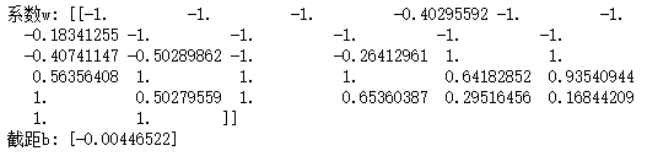
print("系数w:",rbf_svc_moom.named_steps['svc'].dual_coef_)
print("截距b:",rbf_svc_moom.named_steps['svc'].intercept_)
plot_decision_boundary(rbf_svc_moom,axis=[-1.5,2.5,-1.0,1.5])
plt.scatter(x_moom[y_moom==0,0],x_moom[y_moom==0,1])
plt.scatter(x_moom[y_moom==1,0],x_moom[y_moom==1,1])
plt.show()
三、 鸢尾花数据集
iris = datasets.load_iris()

x_iris = iris.data
y_iris = iris.target

x_iris = x_iris [y_iris<2,:2]
y_iris = y_iris[y_iris<2]

plt.scatter(x_iris[y_iris==0,0],x_iris[y_iris==0,1])
plt.scatter(x_iris[y_iris==1,0],x_iris[y_iris==1,1])
plt.show()

- 多项式拟合
poly_svc_iris = PolynomialSVC(degree=5,C=10)

poly_svc_iris.fit(x_iris,y_iris)

print("权重w:",poly_svc_iris.named_steps['linearSVC'].coef_[0])
print("截距b:",poly_svc_iris.named_steps['linearSVC'].intercept_[0])

plot_decision_boundary(poly_svc_iris,axis=[4,7.5,1,4.5])

plt.scatter(x_iris[y_iris==0,0],x_iris[y_iris==0,1])
plt.scatter(x_iris[y_iris==1,0],x_iris[y_iris==1,1])
plt.show()

- 高斯拟合
rbf_svc_iris = RBFKernelSVC(1)

rbf_svc_iris.fit(x_iris,y_iris)

print("系数w:",rbf_svc_iris.named_steps['svc'].dual_coef_)
print("截距b:",rbf_svc_iris.named_steps['svc'].intercept_)

plot_decision_boundary(rbf_svc_iris,axis=[4,7.5,1,4.5])

plt.scatter(x_iris[y_iris==0,0],x_iris[y_iris==0,1])
plt.scatter(x_iris[y_iris==1,0],x_iris[y_iris==1,1])
plt.show()

四、例子重做
import numpy as np
import matplotlib.pyplot as plt
from sklearn import datasets
from sklearn.preprocessing import StandardScaler
from sklearn.svm import LinearSVC
iris = datasets.load_iris()

X = iris.data
y = iris.target

X = X [y<2,:2]
y = y[y<2]

plt.scatter(X[y==0,0],X[y==0,1],color='red')
plt.scatter(X[y==1,0],X[y==1,1],color='blue')
plt.show()

- 高斯核
import numpy as np
import matplotlib.pyplot as plt

x = np.arange(-4,5,1)
y = np.array((x >= -2 ) & (x  2),dtype='int')

plt.scatter(x[y==0],[0]*len(x[y==0]))
plt.scatter(x[y==1],[0]*len(x[y==1]))
plt.show()

def gaussian(x,l):
    gamma = 1.0
    return np.exp(-gamma * (x -l)**2)
l1,l2 = -1,1
X_new = np.empty((len(x),2))
for i,data in enumerate(x):
    X_new[i,0] = gaussian(data,l1)
    X_new[i,1] = gaussian(data,l2)
plt.scatter(X_new[y==0,0],X_new[y==0,1])
plt.scatter(X_new[y==1,0],X_new[y==1,1])
plt.show()


 2万+
2万+


 被折叠的 条评论
为什么被折叠?
被折叠的 条评论
为什么被折叠?
 到【灌水乐园】发言


