


参考:
1、http://docs.opencv.org/3.3.0/ 官方文档api
2、http://docs.opencv.org/3.3.0/d6/d00/tutorial_py_root.html 官方英文教程
3、https://opencv-python-tutroals.readthedocs.io/en/latest/py_tutorials/py_tutorials.html
4、https://github.com/makelove/OpenCV-Python-Tutorial# 进阶教程
5、https://docs.opencv.org/3.3.0/index.html 官方英文教程
6、https://github.com/abidrahmank/OpenCV2-Python-Tutorials
7、https://www.learnopencv.com/
8、http://answers.opencv.org/questions/ OpenCV论坛
注:安装的版本 opencv_python-3.3.0-cp36-cp36m-win_amd64.whl
参考:https://opencv-python-tutroals.readthedocs.io/en/latest/py_tutorials/py_tutorials.html
改变颜色空间
目的
- In this tutorial, you will learn how to convert images from one color-space to another, like BGR
Gray, BGR
- In addition to that, we will create an application which extracts a colored object in a video
- You will learn following functions : cv2.cvtColor(), cv2.inRange() etc.
改变颜色-空间
For BGR Gray conversion we use the flags
cv2.COLOR_BGR2GRAY
. Similarly for BGR
HSV, we use the flag
cv2.COLOR_BGR2HSV
.
>>> import cv2
>>> flags = [i for i in dir(cv2) if i.startswith('COLOR_')]
>>> print flags
For HSV, Hue range is [0,179], Saturation range is [0,255] and Value range is [0,255]. Different softwares use different scales. So if you are comparing OpenCV values with them, you need to normalize these ranges.
对象跟踪
In HSV, it is more easier to represent a color than RGB color-space. In our application, we will try toextracta blue colored object. So here is the method:
- Take each frame of the video
- Convert from BGR to HSV color-space
- We threshold the HSV image for a range of blue color
- Now extract the blue object alone, we can do whatever on that image we want.
import cv2
import numpy as np

# cap = cv2.VideoCapture(0)
cap=cv2.VideoCapture('TownCentreXVID.mp4')

while(1):

    # Take each frame
    _, frame = cap.read()

    # Convert BGR to HSV
    hsv = cv2.cvtColor(frame, cv2.COLOR_BGR2HSV) # 转成HSV

    # define range of blue color in HSV
    lower_blue = np.array([110,50,50])
    upper_blue = np.array([130,255,255])


    # Threshold the HSV image to get only blue colors
    mask = cv2.inRange(hsv, lower_blue, upper_blue)

    # Bitwise-AND mask and original image
    res = cv2.bitwise_and(frame,frame, mask= mask)

    cv2.imshow('frame',frame)
    cv2.imshow('mask',mask)
    cv2.imshow('res',res)
    k = cv2.waitKey(5) & 0xFF
    if k == 27:
        break

cv2.destroyAllWindows()
如何查找HSV值跟踪?
For example, to find the HSV value of Green, try following commands in Python terminal:
>>> green = np.uint8([[[0,255,0 ]]])
>>> hsv_green = cv2.cvtColor(green,cv2.COLOR_BGR2HSV)
>>> print hsv_green
[[[ 60 255 255]]]
Now you take [H-10, 100,100] and [H+10, 255, 255] as lower bound and upper bound respectively.
图像阈值
目标
- In this tutorial, you will learn Simple thresholding, Adaptive thresholding, Otsu’s thresholding etc.
- You will learn these functions : cv2.threshold, cv2.adaptiveThreshold etc.
简单的阈值
- cv2.THRESH_BINARY
- cv2.THRESH_BINARY_INV
- cv2.THRESH_TRUNC
- cv2.THRESH_TOZERO
- cv2.THRESH_TOZERO_INV
import cv2
import numpy as np
from matplotlib import pyplot as plt

img = cv2.imread('lenna.png',0)
ret,thresh1 = cv2.threshold(img,127,255,cv2.THRESH_BINARY)
ret,thresh2 = cv2.threshold(img,127,255,cv2.THRESH_BINARY_INV)
ret,thresh3 = cv2.threshold(img,127,255,cv2.THRESH_TRUNC)
ret,thresh4 = cv2.threshold(img,127,255,cv2.THRESH_TOZERO)
ret,thresh5 = cv2.threshold(img,127,255,cv2.THRESH_TOZERO_INV)

titles = ['Original Image','BINARY','BINARY_INV','TRUNC','TOZERO','TOZERO_INV']
images = [img, thresh1, thresh2, thresh3, thresh4, thresh5]

for i in range(6):
    plt.subplot(2,3,i+1),plt.imshow(images[i],'gray')
    plt.title(titles[i])
    plt.xticks([]),plt.yticks([])

plt.show()
自适应阈值
Adaptive Method - It decides how thresholding value is calculated.- cv2.ADAPTIVE_THRESH_MEAN_C : threshold value is the mean of neighbourhood area.
- cv2.ADAPTIVE_THRESH_GAUSSIAN_C : threshold value is the weighted sum of neighbourhood values where weights are a gaussian window.
C - It is just a constant which is subtracted from the mean or weighted mean calculated.
import cv2
import numpy as np
from matplotlib import pyplot as plt

img = cv2.imread('lenna.png',0)
img = cv2.medianBlur(img,5)

ret,th1 = cv2.threshold(img,127,255,cv2.THRESH_BINARY)
th2 = cv2.adaptiveThreshold(img,255,cv2.ADAPTIVE_THRESH_MEAN_C,\
            cv2.THRESH_BINARY,11,2)
th3 = cv2.adaptiveThreshold(img,255,cv2.ADAPTIVE_THRESH_GAUSSIAN_C,\
            cv2.THRESH_BINARY,11,2)

titles = ['Original Image', 'Global Thresholding (v = 127)',
            'Adaptive Mean Thresholding', 'Adaptive Gaussian Thresholding']
images = [img, th1, th2, th3]

for i in range(4):
    plt.subplot(2,2,i+1),plt.imshow(images[i],'gray')
    plt.title(titles[i])
    plt.xticks([]),plt.yticks([])
plt.show()
Otsu’s 二值化
import cv2
import numpy as np
from matplotlib import pyplot as plt

img = cv2.imread('lenna.png',0)

# global thresholding
ret1,th1 = cv2.threshold(img,127,255,cv2.THRESH_BINARY)

# Otsu's thresholding
ret2,th2 = cv2.threshold(img,0,255,cv2.THRESH_BINARY+cv2.THRESH_OTSU)

# Otsu's thresholding after Gaussian filtering
blur = cv2.GaussianBlur(img,(5,5),0)
ret3,th3 = cv2.threshold(blur,0,255,cv2.THRESH_BINARY+cv2.THRESH_OTSU)

# plot all the images and their histograms
images = [img, 0, th1,
          img, 0, th2,
          blur, 0, th3]
titles = ['Original Noisy Image','Histogram','Global Thresholding (v=127)',
          'Original Noisy Image','Histogram',"Otsu's Thresholding",
          'Gaussian filtered Image','Histogram',"Otsu's Thresholding"]

for i in range(3):
    plt.subplot(3,3,i*3+1),plt.imshow(images[i*3],'gray')
    plt.title(titles[i*3]), plt.xticks([]), plt.yticks([])
    plt.subplot(3,3,i*3+2),plt.hist(images[i*3].ravel(),256)
    plt.title(titles[i*3+1]), plt.xticks([]), plt.yticks([])
    plt.subplot(3,3,i*3+3),plt.imshow(images[i*3+2],'gray')
    plt.title(titles[i*3+2]), plt.xticks([]), plt.yticks([])
plt.show()
Otsu’s二值化化怎样运行?
img = cv2.imread('noisy2.png',0)
blur = cv2.GaussianBlur(img,(5,5),0)

# find normalized_histogram, and its cumulative distribution function
hist = cv2.calcHist([blur],[0],None,[256],[0,256])
hist_norm = hist.ravel()/hist.max()
Q = hist_norm.cumsum()

bins = np.arange(256)

fn_min = np.inf
thresh = -1

for i in xrange(1,256):
    p1,p2 = np.hsplit(hist_norm,[i]) # probabilities
    q1,q2 = Q[i],Q[255]-Q[i] # cum sum of classes
    b1,b2 = np.hsplit(bins,[i]) # weights

    # finding means and variances
    m1,m2 = np.sum(p1*b1)/q1, np.sum(p2*b2)/q2
    v1,v2 = np.sum(((b1-m1)**2)*p1)/q1,np.sum(((b2-m2)**2)*p2)/q2

    # calculates the minimization function
    fn = v1*q1 + v2*q2
    if fn < fn_min:
        fn_min = fn
        thresh = i

# find otsu's threshold value with OpenCV function
ret, otsu = cv2.threshold(blur,0,255,cv2.THRESH_BINARY+cv2.THRESH_OTSU)
print thresh,ret
图像的几何变换
目标
- Learn to apply different geometric transformation to images like translation, rotation, affine transformation etc.
- You will see these functions: cv2.getPerspectiveTransform
转换
缩放
Scaling is just resizing of the image.cv2.resize()Preferable interpolation methods are cv2.INTER_AREA for shrinking and cv2.INTER_CUBIC (slow) & cv2.INTER_LINEAR for zooming. By default, interpolation method used is cv2.INTER_LINEAR for all resizing purposes.
import cv2
import numpy as np

img = cv2.imread('messi5.jpg')

res = cv2.resize(img,None,fx=2, fy=2, interpolation = cv2.INTER_CUBIC)

#OR

height, width = img.shape[:2]
res = cv2.resize(img,(2*width, 2*height), interpolation = cv2.INTER_CUBIC)
翻动
import cv2
import numpy as np

img = cv2.imread('messi5.jpg',0)
rows,cols = img.shape

M = np.float32([[1,0,100],[0,1,50]])
dst = cv2.warpAffine(img,M,(cols,rows))

cv2.imshow('img',dst)
cv2.waitKey(0)
cv2.destroyAllWindows()
Third argument of the cv2.warpAffine() function is the size of the output image, which should be in the form of (width, height) . Remember width = number of columns, and height = number of rows.
旋转
import cv2

img = cv2.imread('messi5.jpg',0)
rows,cols = img.shape

M = cv2.getRotationMatrix2D((cols/2,rows/2),90,1) # 逆时针旋转90度
dst = cv2.warpAffine(img,M,(cols,rows))

cv2.imshow('dst',dst)
cv2.waitKey(0)
cv2.destroyAllWindows()
仿射变换
Then cv2.getAffineTransform will create a 2x3 matrix which is to be passed to cv2.warpAffine .
import cv2
import numpy as np
import matplotlib.pyplot as plt

img = cv2.imread('lenna.png')
rows,cols,ch = img.shape

pts1 = np.float32([[50,50],[200,50],[50,200]])
pts2 = np.float32([[10,100],[200,50],[100,250]])

M = cv2.getAffineTransform(pts1,pts2)

dst = cv2.warpAffine(img,M,(cols,rows))

plt.subplot(121),plt.imshow(img),plt.title('Input')
plt.subplot(122),plt.imshow(dst),plt.title('Output')
plt.show()
透视转换
Then transformation matrix can be found by the functioncv2.getPerspectiveTransform. Then apply cv2.warpPerspective with this 3x3 transformation matrix.
import cv2
import numpy as np
import matplotlib.pyplot as plt

img = cv2.imread('lenna.png')
rows,cols,ch = img.shape

pts1 = np.float32([[56,65],[368,52],[28,387],[389,390]])
pts2 = np.float32([[0,0],[300,0],[0,300],[300,300]])

M = cv2.getPerspectiveTransform(pts1,pts2)

dst = cv2.warpPerspective(img,M,(300,300))

plt.subplot(121),plt.imshow(img),plt.title('Input')
plt.subplot(122),plt.imshow(dst),plt.title('Output')
plt.show()
平滑图像
目标
-
Learn to:
-
- Blur imagess with various low pass filters
- Apply custom-made filters to images (2D convolution)
二维卷积(图像过滤)
import cv2
import numpy as np
from matplotlib import pyplot as plt

img = cv2.imread('opencv_logo.png')

kernel = np.ones((5,5),np.float32)/25
dst = cv2.filter2D(img,-1,kernel)

plt.subplot(121),plt.imshow(img),plt.title('Original')
plt.xticks([]), plt.yticks([])
plt.subplot(122),plt.imshow(dst),plt.title('Averaging')
plt.xticks([]), plt.yticks([])
plt.show()
图像模糊(图像平滑)
1. 均值滤波
This is done by the function cv2.blur() or cv2.boxFilter()If you don’t want to use a normalized box filter, use cv2.boxFilter() and pass the argumentnormalize=False to the function.
import cv2
import numpy as np
from matplotlib import pyplot as plt

img = cv2.imread('opencv_logo.png')

blur = cv2.blur(img,(5,5))

plt.subplot(121),plt.imshow(img),plt.title('Original')
plt.xticks([]), plt.yticks([])
plt.subplot(122),plt.imshow(blur),plt.title('Blurred')
plt.xticks([]), plt.yticks([])
plt.show()
2. 高斯滤波
If you want, you can create a Gaussian kernel with the function, cv2.getGaussianKernel().
import cv2
import numpy as np
from matplotlib import pyplot as plt

img = cv2.imread('opencv_logo.png')

# blur = cv2.blur(img,(5,5))
blur = cv2.GaussianBlur(img,(5,5),0)

plt.subplot(121),plt.imshow(img),plt.title('Original')
plt.xticks([]), plt.yticks([])
plt.subplot(122),plt.imshow(blur),plt.title('Blurred')
plt.xticks([]), plt.yticks([])
plt.show()
3. 中值滤波
cv2.medianBlur()
median = cv2.medianBlur(img,5)
4. 双边过滤
cv2.bilateralFilter() ,
blur = cv2.bilateralFilter(img,9,75,75)
Additional Resources
- Details about the bilateral filtering can be found at
形态转化
目标
-
In this chapter,
-
- We will learn different morphological operations like Erosion, Dilation, Opening, Closing etc.
- We will see different functions like : cv2.erode(), cv2.dilate(), cv2.morphologyEx() etc.
理论
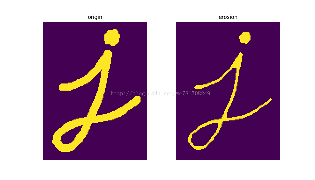
它通常是操作二进制图像。需要两个输入,一个是原始影像,一个是structuring element or kernel。两个基本形态操作是腐蚀和膨胀1. Erosion(腐蚀)
腐蚀前景的边界(总是尝试保持前景为白色)。内核滑过图像(如2D卷积)。只有当内核下的所有像素为1时,才能将原始图像(1或0)中的像素视为1,否则将被侵蚀(使为零)。
取决于内核的大小,边界附近的所有像素将被丢弃。因此,前景对象的厚度或尺寸减小,或者仅仅是图像中的白色区域减小。它有助于去除小白噪声(如我们在颜色空间章节中看到的),分离两个连接的对象等。
Here, as an example, I would use a 5x5 kernel with full of ones. Let’s see it how it works:
import cv2
import numpy as np
import matplotlib.pyplot as plt

img = cv2.imread('j.png',0)
kernel = np.ones((5,5),np.uint8)
erosion = cv2.erode(img,kernel,iterations = 1)

plt.subplot(121);plt.imshow(img);plt.title('origin');plt.axis('off')
plt.subplot(122);plt.imshow(erosion);plt.title('erosion');plt.axis('off')
plt.show()
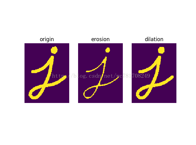
2. Dilation(膨胀)
与腐蚀刚好相反。一个像素元素是' 1 '如果至少一个像素在内核是“1”。所以它增加了白色地区前景物体的图像或尺寸增加。通常,在噪声去除情况下,侵蚀是紧随其后的扩张。因为,侵蚀去除白噪声,但也减少我们的对象。所以我们扩张。因为噪音消失了,他们不会回来,但我们的对象面积增加。也有用的加入打破地区的一个对象。
import cv2
import numpy as np
import matplotlib.pyplot as plt

img = cv2.imread('j.png',0)
kernel = np.ones((5,5),np.uint8)  # 内核
erosion = cv2.erode(img,kernel,iterations = 1)  # 腐蚀去除噪声
dilation = cv2.dilate(erosion,kernel,iterations = 1) # 膨胀恢复原形状

plt.subplot(131);plt.imshow(img);plt.title('origin');plt.axis('off')
plt.subplot(132);plt.imshow(erosion);plt.title('erosion');plt.axis('off')
plt.subplot(133);plt.imshow(dilation);plt.title('dilation');plt.axis('off')
plt.show()
3. 开运算
Opening只是另一个侵蚀的名字,随后是扩张。是有用的在去除噪声,正如我们上面的解释。
Here we use the function,
cv2.morphologyEx()
import cv2
import numpy as np
import matplotlib.pyplot as plt

img = cv2.imread('j.png',0)
kernel = np.ones((5,5),np.uint8)  # 内核
erosion = cv2.erode(img,kernel,iterations = 1)  # 腐蚀去除噪声
dilation = cv2.dilate(erosion,kernel,iterations = 1) # 膨胀恢复原形状

opening = cv2.morphologyEx(img, cv2.MORPH_OPEN, kernel)
dilation2 = cv2.dilate(opening,kernel,iterations = 1) # 膨胀恢复原形状


plt.subplot(231);plt.imshow(img);plt.title('origin');plt.axis('off')
plt.subplot(232);plt.imshow(erosion);plt.title('erosion');plt.axis('off')
plt.subplot(233);plt.imshow(dilation);plt.title('dilation');plt.axis('off')

plt.subplot(234);plt.imshow(opening);plt.title('opening');plt.axis('off')
plt.subplot(235);plt.imshow(dilation2);plt.title('dilation2');plt.axis('off')
plt.show()

4. 闭运算
封闭与开放相反,扩张之后是侵蚀。是有用的在关闭小洞内的前景对象,对象或黑色小点。
closing = cv2.morphologyEx(img, cv2.MORPH_CLOSE, kernel)
5. 形态梯度
图像的扩张和侵蚀的区别。gradient = cv2.morphologyEx(img, cv2.MORPH_GRADIENT, kernel)
6. 顶帽
tophat = cv2.morphologyEx(img, cv2.MORPH_TOPHAT, kernel)
7. 黑帽
输入图像和输入图像的
closing 是不同的。
blackhat = cv2.morphologyEx(img, cv2.MORPH_BLACKHAT, kernel)
结构元素
在Numpy的帮助下,我们在前面的例子中手动创建了一个结构化元素。 它是矩形的。 但是在某些情况下,您可能需要椭圆/圆形的内核。 所以为了这个目的,OpenCV有一个函数 cv2.getStructuringElement()。 你只是传递内核的形状和大小,你会得到所需的内核。# Rectangular Kernel
>>> cv2.getStructuringElement(cv2.MORPH_RECT,(5,5))
array([[1, 1, 1, 1, 1],
[1, 1, 1, 1, 1],
[1, 1, 1, 1, 1],
[1, 1, 1, 1, 1],
[1, 1, 1, 1, 1]], dtype=uint8)
# Elliptical Kernel
>>> cv2.getStructuringElement(cv2.MORPH_ELLIPSE,(5,5))
array([[0, 0, 1, 0, 0],
[1, 1, 1, 1, 1],
[1, 1, 1, 1, 1],
[1, 1, 1, 1, 1],
[0, 0, 1, 0, 0]], dtype=uint8)
# Cross-shaped Kernel
>>> cv2.getStructuringElement(cv2.MORPH_CROSS,(5,5))
array([[0, 0, 1, 0, 0],
[0, 0, 1, 0, 0],
[1, 1, 1, 1, 1],
[0, 0, 1, 0, 0],
[0, 0, 1, 0, 0]], dtype=uint8)
Additional Resources
- Morphological Operations at HIPR2
图像梯度
目标
In this chapter, we will learn to:
- Find Image gradients, edges etc
- We will see following functions : cv2.Sobel(), cv2.Scharr(), cv2.Laplacian() etc
理论
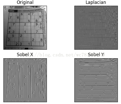
OpenCV提供三种类型的梯度滤波器或高通滤波器,Sobel,Scharr和Laplacian。 我们会看到他们中的每一个。
1. Sobel 和 Scharr 导数
Sobel操作是高斯平滑加分散操作的联合,因此更能抵抗噪音。 您可以指定要采取的导数的方向,垂直方向或水平方向(分别为参数yorder和xorder)。 您还可以通过参数ksize指定内核的大小。 如果ksize = -1,则使用3x3 Scharr滤波器,该滤波器比3x3 Sobel滤波器更好的结果。 请参阅使用的内核文档。
2. 拉普拉斯导数
它计算由关系给出的图像的拉普拉斯算子, 这里每一个导数都使用了Sobel导数。如果ksize = 1,则使用以下内核进行过滤:

代码
以下代码显示了单个图中的所有运算符。 所有内核的大小为5x5。 输出图像的深度通过-1来获得np.uint8类型的结果。
import cv2
import numpy as np
from matplotlib import pyplot as plt

img = cv2.imread('dave.jpg',0)

laplacian = cv2.Laplacian(img,cv2.CV_64F)
sobelx = cv2.Sobel(img,cv2.CV_64F,1,0,ksize=5)
sobely = cv2.Sobel(img,cv2.CV_64F,0,1,ksize=5)

plt.subplot(2,2,1),plt.imshow(img,cmap = 'gray')
plt.title('Original'), plt.xticks([]), plt.yticks([])
plt.subplot(2,2,2),plt.imshow(laplacian,cmap = 'gray')
plt.title('Laplacian'), plt.xticks([]), plt.yticks([])
plt.subplot(2,2,3),plt.imshow(sobelx,cmap = 'gray')
plt.title('Sobel X'), plt.xticks([]), plt.yticks([])
plt.subplot(2,2,4),plt.imshow(sobely,cmap = 'gray')
plt.title('Sobel Y'), plt.xticks([]), plt.yticks([])

plt.show()
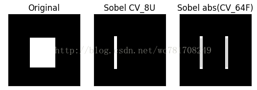
一个重要的事项!
在我们的最后一个例子中,输出数据类型是cv2.CV_8U或np.uint8。 但是有一个小问题。 将黑白转换作为正斜率(它具有正值),而将白 - 黑转换作为负斜率(它具有负值)。 所以当你将数据转换为np.uint8时,所有的负斜率均为零。 简单来说,你错过了这个边缘。如果要检测到这两个边,更好的选择是将输出数据类型保持为一些较高的形式,如cv2.CV_16S,cv2.CV_64F等,取其绝对值,然后转换回cv2.CV_8U。 下面的代码演示了水平Sobel滤波器的这个过程以及结果的差异。
import cv2
import numpy as np
from matplotlib import pyplot as plt

img = cv2.imread('box.png',0)

# Output dtype = cv2.CV_8U
sobelx8u = cv2.Sobel(img,cv2.CV_8U,1,0,ksize=5)

# Output dtype = cv2.CV_64F. Then take its absolute and convert to cv2.CV_8U
sobelx64f = cv2.Sobel(img,cv2.CV_64F,1,0,ksize=5)
abs_sobel64f = np.absolute(sobelx64f)
sobel_8u = np.uint8(abs_sobel64f)

plt.subplot(1,3,1),plt.imshow(img,cmap = 'gray')
plt.title('Original'), plt.xticks([]), plt.yticks([])
plt.subplot(1,3,2),plt.imshow(sobelx8u,cmap = 'gray')
plt.title('Sobel CV_8U'), plt.xticks([]), plt.yticks([])
plt.subplot(1,3,3),plt.imshow(sobel_8u,cmap = 'gray')
plt.title('Sobel abs(CV_64F)'), plt.xticks([]), plt.yticks([])

plt.show()
Canny边缘检测
目标
In this chapter, we will learn about
- Concept of Canny edge detection
- OpenCV functions for that : cv2.Canny()
理论
- 降噪
由于边缘检测对图像中的噪声敏感,所以第一步是用5x5高斯滤波器去除图像中的噪声。 我们已经在前几章看到过。
- 寻找图像的强度梯度

梯度方向始终垂直于边缘。 它被四舍五入为表示垂直,水平和两个对角线方向的四个角度之一。
- 非最大抑制

点A位于边缘(垂直方向)。 梯度方向与边缘正交。 点B和C处于梯度方向。 点B和C检查点A是否形成局部最大值。 如果是这样,则考虑下一阶段,否则被抑制(置零)。
简而言之,您获得的结果是具有“薄边”的二进制图像。
- 滞后阈值

边缘A在maxVal之上,因此被视为“肯定边缘”。 虽然边缘C低于maxVal,但它连接到边缘A,因此也被认为是有效边缘,并且我们得到该完整曲线。 但边缘B虽然高于minVal并且与边缘C的区域相同,但是它没有连接到任何“肯定边缘”,因此被丢弃。 所以非常重要的是我们必须相应地选择minVal和maxVal才能得到正确的结果。
假设边缘是长线,这个阶段也会消除小像素的噪音。
所以我们终于得到的是图像中的强势。
OpenCV中的Canny边缘检测
OpenCV将以上所有内容放在单个函数 cv2.Canny()中。 我们将看到如何使用它。 第一个参数是我们的输入图像。 第二和第三个参数分别是我们的minVal和maxVal。 第三个参数是aperture_size。 用于查找图像渐变的Sobel内核的大小。 默认情况下是3。最后一个参数是L2gradient,它指定查找梯度大小的方程。 如果为True,则使用上述等式更准确,否则使用此函数: 。 默认情况下,它是False。
import cv2
import numpy as np
from matplotlib import pyplot as plt

img = cv2.imread('messi5.jpg',0)
edges = cv2.Canny(img,100,200)

plt.subplot(121),plt.imshow(img,cmap = 'gray')
plt.title('Original Image'), plt.xticks([]), plt.yticks([])
plt.subplot(122),plt.imshow(edges,cmap = 'gray')
plt.title('Edge Image'), plt.xticks([]), plt.yticks([])

plt.show()

Additional Resources
- Canny edge detector at Wikipedia
- Canny Edge Detection Tutorial by Bill Green, 2002.
图像金字塔
目标
-
In this chapter,
-
- We will learn about Image Pyramids
- We will use Image pyramids to create a new fruit, “Orapple”
- We will see these functions: cv2.pyrUp(), cv2.pyrDown()
理论
通常,我们曾经使用一个恒定大小的图像。 但在某些情况下,我们需要处理相同图像的不同分辨率的图像。 例如,在像图像中寻找某物的同时,我们不确定图像中的对象将以什么大小显示。 在这种情况下,我们将需要创建一组不同分辨率的图像,并在所有图像中搜索对象。 这些具有不同分辨率的图像被称为图像金字塔(因为当它们保持在堆叠中,最大图像在底部,最小图像在顶部看起来像金字塔)。
有两种图像金字塔。 1)高斯金字塔和2)拉普拉斯金字塔
高斯金字塔中的较高级别(低分辨率)是通过删除较低级别(较高分辨率)图像中的连续行和列来形成的。 然后,较高级别中的每个像素由基础级别中的5个像素与高斯权重的贡献形成。 通过这样做,  图像成为
图像成为  图像。 因此,面积减少到原始面积的四分之一。 它被称为八度。 我们在金字塔上升(即分辨率降低)时,相同的模式继续下去。 类似地,在扩展时,每个层面的面积变成4倍。 我们可以使用cv2.pyrDown() and cv2.pyrUp()函数找到高斯金字塔。
img = cv2.imread('messi5.jpg')
lower_reso = cv2.pyrDown(higher_reso)
Now you can go down the image pyramid with cv2.pyrUp() function.
higher_reso2 = cv2.pyrUp(lower_reso)记住,higher_reso2不等于higher_reso,因为一旦你降低了分辨率,你会丢失信息。 在以前的情况下,图像是从最小图像创建的金字塔3级。 与原始图像进行比较:
拉普拉斯金字塔由高斯金字塔形成。 没有排他的功能。 拉普拉斯金字塔图像仅仅是边缘图像。 它的大多数元素都是零。 它们用于图像压缩。 拉普拉斯金字塔中的一个层次是由高斯金字塔的高低与高斯金字塔上层扩展版本之间的差异形成的。 拉普拉斯等级的三个级别将如下所示(对比度被调整以增强内容):
使用金字塔的图像混合
金字塔的一个应用是图像混合。 例如,在图像拼接中,您需要将两个图像堆叠在一起,但由于图像之间的不连续性,它可能看起来不太好。 在这种情况下,与金字塔的图像混合可以让您无缝混合,而不会在图像中留下大量数据。 一个典型的例子就是混合了两种水果,橙子和苹果。 现在看看结果来了解我在说什么:
- 加载苹果和橙色的两个图像
- 找到苹果和橙色的高斯金字塔(在这个特殊的例子中,数量是6)
- 从高斯金字塔,找到他们的拉普拉斯金字塔
- 现在加入苹果的左半部分,在拉普拉斯金字塔各个级别的橙子右半部分
- 最后从这个联合图像金字塔,重建原始的形象。
import cv2
import numpy as np,sys

A = cv2.imread('apple.jpg')
B = cv2.imread('orange.jpg')

# generate Gaussian pyramid for A
G = A.copy()
gpA = [G]
for i in range(6):
    G = cv2.pyrDown(G)
    gpA.append(G)

# generate Gaussian pyramid for B
G = B.copy()
gpB = [G]
for i in range(6):
    G = cv2.pyrDown(G)
    gpB.append(G)

# generate Laplacian Pyramid for A
lpA = [gpA[5]]
for i in range(5,0,-1):
    GE = cv2.pyrUp(gpA[i])
    L = cv2.subtract(gpA[i-1],GE)
    lpA.append(L)

# generate Laplacian Pyramid for B
lpB = [gpB[5]]
for i in range(5,0,-1):
    GE = cv2.pyrUp(gpB[i])
    L = cv2.subtract(gpB[i-1],GE)
    lpB.append(L)

# Now add left and right halves of images in each level
LS = []
for la,lb in zip(lpA,lpB):
    rows,cols,dpt = la.shape
    ls = np.hstack((la[:,0:cols//2], lb[:,cols//2:]))
    LS.append(ls)

# now reconstruct
ls_ = LS[0]
for i in range(1,6):
    ls_ = cv2.pyrUp(ls_)
    ls_ = cv2.add(ls_, LS[i])

# image with direct connecting each half
real = np.hstack((A[:,:cols//2],B[:,cols//2:]))

cv2.imwrite('Pyramid_blending2.jpg',ls_)
cv2.imwrite('Direct_blending.jpg',real)

cv2.imshow('Pyramid_blending2',ls_)
cv2.imshow('Direct_blending',real)
cv2.waitKey(0)
cv2.destroyAllWindows()
Additional Resources


 668
668

 被折叠的 条评论
为什么被折叠?
被折叠的 条评论
为什么被折叠?
 到【灌水乐园】发言


