


深度学习分类pytorch
立即学习AI (Learn AI Today)
This is the second story in the Learn AI Today series I’m creating! These stories, or at least the first few, are based on a series of Jupyter notebooks I’ve created while studying/learning PyTorch and Deep Learning. I hope you find them as useful as I did!
这是《 今日学习AI》中的第二个故事 我正在创建的系列! 这些故事,或者至少是前几篇小说,是基于我在学习/学习PyTorch和Deep Learning时创建的一系列Jupyter笔记本的 。 希望您发现它们和我一样有用!
If you have not already, make sure to check the previous story!
如果您还没有,请确保检查以前的故事!
您将从这个故事中学到什么: (What you will learn in this story:)
- The Importance of Validation 验证的重要性
- How to Train Models for Classification Problems 如何为分类问题训练模型
- Visualize the Decision Boundaries Dynamically 动态可视化决策边界
- How to Avoid Overfitting 如何避免过度拟合
1.鸢尾花数据集 (1. Iris Flower Dataset)
Let’s get started by introducing the dataset. I will be using the very famous Iris flower dataset that contains 4 different measurements (sepal length, sepal width, petal length, petal width) of the following 3 species of flowers.
让我们开始介绍数据集。 我将使用非常著名的鸢尾花数据集 ,该数据集包含以下3种花的4种不同测量值(花冠长度,萼片宽度,花瓣长度,花瓣宽度)。

The goal is to accurately identify the species using the 4 measurements for each flower. Note that nowadays it’s relatively easy to use a model (Convolutional Neural Networks) that learns directly from the images but I will leave that topic for the next lesson. The Iris flower dataset can be easily downloaded from sklearn datasets as shown in the code below.
目标是使用每朵花的4个测量值来准确识别物种。 请注意,如今使用直接从图像中学习的模型(卷积神经网络)相对容易,但是我将把该主题留给下一课。 的鸢尾花数据集可以如下图所示的代码可以容易地从数据集sklearn下载。
To get a quick visualization of the data let’s plot the scatter plots of each pair of features and the histograms for each feature. To achieve this representation I used the pandas.plotting.scatter_matrix function (as always you can find the link to the full code at the end).
为了快速查看数据,让我们绘制每对特征的散点图和每个特征的直方图。 为了实现这种表示,我使用了pandas.plotting.scatter_matrix函数(一如既往,您可以在最后找到完整代码的链接)。
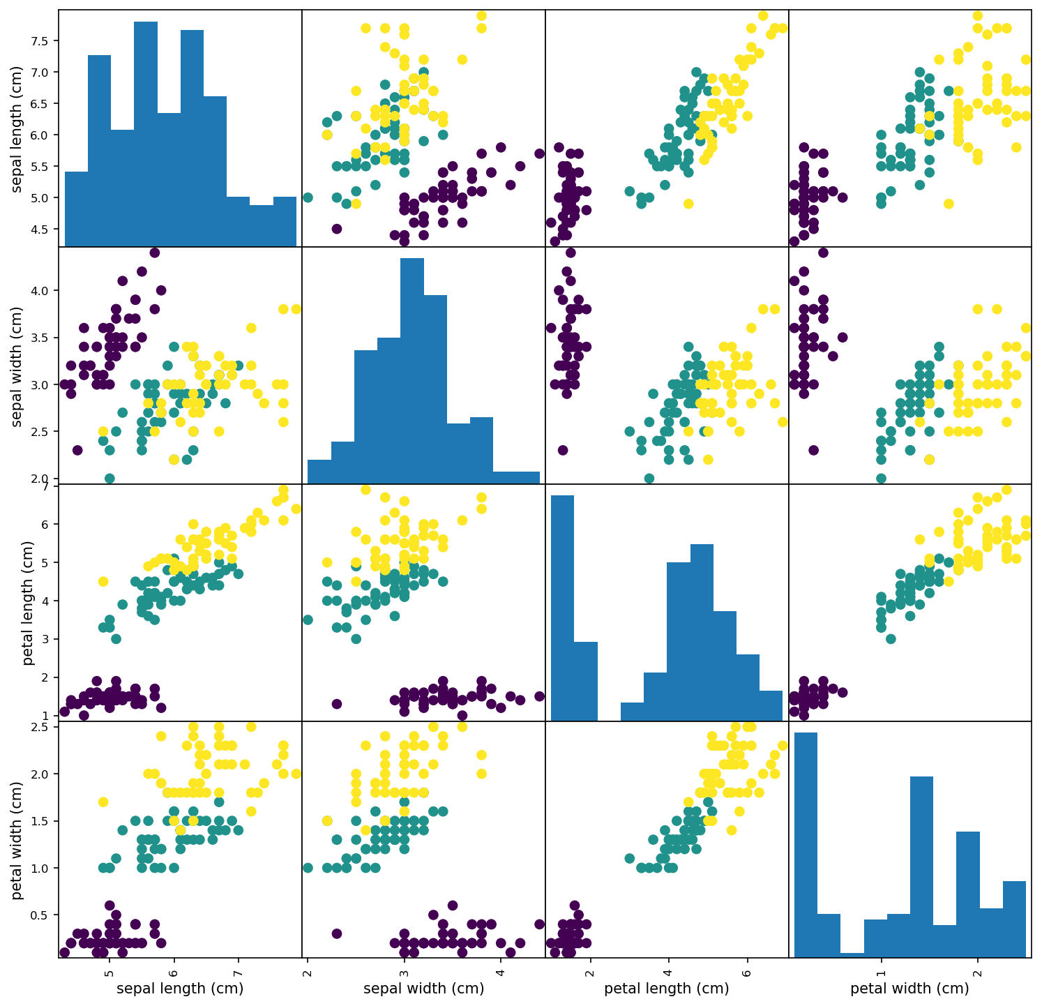
As you can see on the scatter plots above, for most of the samples it should be easy to discriminate the specie. For example, the Iris setosa dots are, in most plots, very well separated from the other two species. For such an easy example you can easily create a rule-based algorithm by drawing a few lines. However, for its simplicity, is also a good example to introduce classification with Neural Networks!
正如您在上面的散点图上看到的那样,对于大多数样本来说,应该容易区分物种。 例如,在大多数小区中, 鸢尾鸢尾花点与其他两个物种之间的距离非常好。 对于这样一个简单的示例,您可以通过画几条线来轻松创建基于规则的算法 。 但是,为简单起见,它也是在 神经网络中引入分类的 一个很好的例子 !
2.验证集 (2. Validation Set)
Before jumping straight to the models and training it’s very important to create a validation set. I skipped this step in the first lesson to avoid introducing too many concepts all at once.
在直接进入模型并进行训练之前,创建验证集非常重要 。 在第一课中,我跳过了这一步,以避免一次引入太多概念。
The idea of a validation set is simple. Instead of training a model with all your data you put apart a fraction of the data (usually 20% — 30%) that you will use to evaluate if the trained model generalizes well to unseen data. This is very important to make sure your model can be safely put into production to evaluate new data accurately.
验证集的想法很简单。 无需使用所有数据来训练模型,而是将一部分数据 (通常为20%-30%) 分开,这些数据将用于评估训练后的模型是否可以很好地推广到看不见的数据 。 这对于确保您的模型可以安全地投入生产以准确评估新数据非常重要。
In the code above I make use of train_test_split function to randomly split the data and I choose a test_size=0.5 . It’s always a good idea to set the random_state to make sure that when you re-run the code the same split will be used.
在上面的代码中,我使用train_test_split函数随机分割数据,然后选择test_size=0.5 。 设置random_state始终是一个好主意,以确保当您重新运行代码时,将使用相同的拆分。
Notice that it is common and a good practice two have not 2 but 3 data splits: train, validation and test. In that case, you use the validation set to check the progress when you try several models, ideas and hyper-parameters (e.g. the learning rate) and you only use the test set at the end when you are happy with the results. This is what happens in Kaggle competitions where usually there is a hidden test set.
请注意,这是一种常见的习惯做法,两个不是2 个数据而是3个数据拆分:train,validation和test 。 在这种情况下,当您尝试几种模型,想法和超参数(例如学习率)时,可以使用验证集检查进度,并且只有对结果满意时才使用测试集。 这就是在Kaggle比赛中发生的情况,通常会有一个隐藏的测试集 。
3.训练分类模型 (3. Training a Model for Classification)
The model I’m going to use for this example is exactly the same I used in the previous lesson for the regression problems!
我将在此示例中使用的模型与上一课中关于回归问题的模型完全相同!
So what’s the difference? The difference is in the loss function. For multi-class classification problems, the usual choice is Cross Entropy Loss (nn.CrossEntropyLoss in PyTorch). For binary classification problems, you usually use Binary Cross Entropy Loss (nn.BCEWithLogitsLoss). As a result, the code for defining the model, criterion and optimizer is very similar to what I used in the previous lesson for regression!
那有什么区别呢? 区别在于损失函数 。 对于多类别分类问题,通常的选择是交叉熵损失 (PyTorch中的nn.CrossEntropyLoss)。 对于二进制分类问题,通常使用二进制交叉熵 损失 (nn.BCEWithLogitsLoss)。 结果,用于定义模型,标准和优化器的代码与我在上一课中进行回归的代码非常相似!
An additional difference to consider is the last activation function. For regression problems, the output of the model is a number that can be any real value. For binary classification, you need to use a Sigmoid activation function that maps the output to the 0–1 range. For multi-class classification you need Softmax activation function (unless you want to allow for multiple choices, in that case use Sigmoid activation). The Softmax output can be interpreted as the probability assigned to each class.
要考虑的另一个区别是最后一个激活功能。 对于回归问题,模型的输出是可以是任何实际值的数字。 对于二进制分类 ,您需要使用Sigmoid激活函数 ,将输出映射到0–1范围。 对于多类别分类,您需要Softmax激活功能 (除非您希望允许多个选择,在这种情况下,请使用Sigmoid激活)。 Softmax输出可以解释为分配给每个类别的概率。
Don’t worry too much for now about the activation functions. I’m just mentioning it here so that you are aware of their existence. For now, the good thing to know is that nn.CrossEntropyLoss includes the Softmax activation for you and the nn.BCEWithLogitsLoss includes the Sigmoid for you. That way you don’t need to add any activation function at the end of the model. PyTorch takes care of that for you!
现在不用担心激活功能。 我只是在这里提到它,以便您知道它们的存在。 现在,您要知道的是, nn.CrossEntropyLoss为您提供了Softmax激活,而nn.BCEWithLogitsLoss为您提供了Sigmoid。 这样,您无需在模型末尾添加任何激活功能。 PyTorch会为您解决这个问题!
Before training the model I also changed the fit function from the previous lesson (you can check it in the Kaggle notebook with the complete code at the end) to allow for train and test/validation data. (When working with only two datasets the terms validation and test are often used interchangeably.)
在训练模型之前,我还更改了上一课的fit函数(您可以在Kaggle笔记本中检查它的末尾带有完整的代码)以允许train和test/validation数据。 (当仅使用两个数据集时, 验证和测试一词经常互换使用。)
Plotting the losses for train and test during the 1000 epochs of training you can see something weird is going on.
绘制1000次训练期间的训练和测试损失图,您会看到奇怪的事情在发生 。
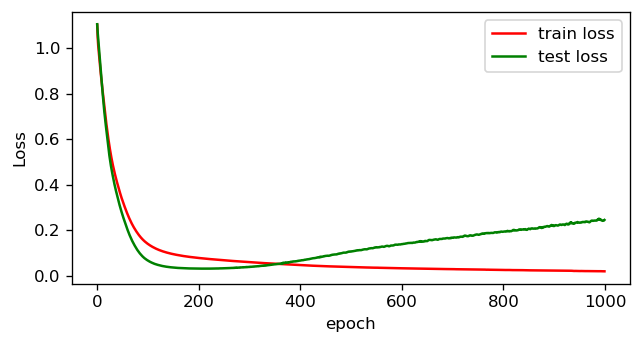
While the train loss keeps improving over time, the test loss initially improves steadily but then starts to increase. And perhaps most importantly, you can see the same effect by plotting the accuracy of the model over the 1000 epochs.
虽然火车损耗随着时间的流逝而不断改善,但测试损耗最初稳定地提高,但随后开始增加 。 也许最重要的是,通过在1000个时期内绘制模型的准确性 , 您可以看到相同的效果 。
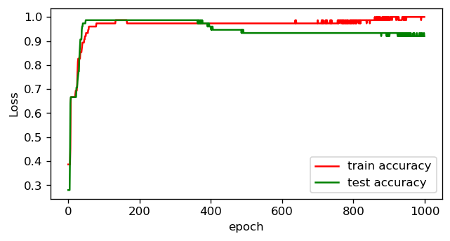
What you are seeing is what we call overfitting — at some point the model starts ‘remembering’ the train data and the generalization performance (evaluated with the test set) decreases. And that’s why you need a validation/test set. In this case you can see that possibly the results are better if you stop the training at 200 epochs. This method is called early stopping and is an easy way to reduce overfitting. However there are other ways such as using weight decay that I will talk about in a minute. Let’s first do some fun visualizations to understand better what is going.
您所看到的就是我们所说的过拟合 -在 在某个点上,模型开始“记住”列车数据, 泛化性能 (用测试集评估) 降低 。 这就是为什么您需要验证/测试集。 在这种情况下,您可以看到,如果您停止训练200个纪元,结果可能会更好。 这种方法称为提前停止 ,是减少过度拟合的一种简便方法。 但是,还有其他方法,例如使用重量衰减 ,我将在稍后讨论。 首先,让我们做一些有趣的可视化,以更好地了解正在发生的事情。
4.可视化决策边界并减少过度拟合 (4. Visualizing Decision Boundaries and Reducing Overfitting)
To visualize the training boundaries and better understand overfitting, I retrained the model using only 2 (instead of 4) features in order to easily plot the result in a 2D graphic. In the animation below you can see the decision boundaries for train (left) and test (right) evolving during the 1000 training epochs.
为了可视化训练边界并更好地理解过度拟合,我仅使用2个(而不是4个)特征对模型进行了重新训练,以便轻松地在2D图形中绘制结果。 在下面的动画中,您可以看到在1000个训练时期内训练(左)和测试(右)的决策边界。
Look how initially the model quickly learns 2 straight line boundaries dividing the regions. Then, the red-yellow boundary starts to curve upwards, adjusting better to the train set. However, looking at the test set this leads to a slight decrease in performance as more yellow dots move to the middle region and green-bluish dots to the top region. And this is exactly what overfitting looks like. For more complex problems you can imagine this in multiple dimensions — it’s easier to overfit when you have a lot of dimensions.
看看模型最初是如何快速学习2条划分区域的直线边界的。 然后, 红黄色边界开始向上弯曲 ,从而更好地适应了列车的设置。 但是,查看测试集会导致性能略有下降,因为更多的黄色点移到中间区域,绿色蓝色点移到顶部区域。 这正是过度拟合的样子 。 对于更复杂的问题,您可以在多个维度上进行想象-当您拥有多个维度时 ,更容易过度拟合。
If you have trouble imagining anything in more than 3 dimensions just follow this advice from Geoffrey Hinton: “To deal with hyper-planes in a 14-dimensional space, visualize a 3-D space and say ‘fourteen’ to yourself very loudly. Everyone does it.”
如果您无法想象3维以上的物体,请遵循Geoffrey Hinton的建议: “要处理14维空间中的超平面,请可视化3D空间并大声地对自己说“十四”。 每个人都做。”
To reduce overfitting in this example you can use two simple ‘tricks’:
为了减少过度拟合,您可以使用两个简单的“技巧”:
Early Stopping: Train the model for fewer epochs
尽早停止:训练模型的时间更少
Weight Decay: Force the model weights to be small by reducing them by a small amount each iteration
权重衰减:通过在每次迭代中将模型权重减少少量来强制减小模型权重
4.1提前停止 (4.1 Early Stopping)
The idea of Early Stopping is very simple, as I mentioned before if the model has the best validation accuracy at around epoch 200 then if you train for only 200 epochs you will get a model that generalizes better — according to the validation accuracy. The problem is that you may then be visually overfitting to the validation set — particularly if you tune a lot of hyperparameters based on the validation score. This is why it’s often important to have an additional set of data to evaluate the model after finishing all the experiments.
提前停止的想法非常简单,正如我之前提到的,如果模型在约200个时期具有最佳的验证准确性,那么如果仅训练200个时期,则根据验证准确性,您将得到一个概括性更好的模型。 问题在于您可能随后在视觉上过度适应了验证集-尤其是如果您根据验证得分调整了许多超参数。 这就是为什么在完成所有实验后拥有一组额外的数据来评估模型通常很重要的原因。
4.2重量衰减 (4.2 Weight Decay)
The idea of Weight Decay is also simple. When fitting a Neural Network, in general, there isn’t an optimum solution but multiple possible similar solutions. Weight Decay, by forcing the weights to stay small, will force the optimization process to reach a simpler solution.
重量衰减的想法也很简单。 通常,在安装神经网络时,没有最佳解决方案,但有多种可能的类似解决方案。 通过迫使权重保持较小,权重衰减将迫使优化过程达到更简单的解决方案。
Let’s add a weight_decay=0.01 to our model and visualize the results after training for 1000 epochs as before. In PyTorch, you just need to add this parameter to the optimizer as optimizer = optim.Adam(model.parameters, lr=0.001, weight_decay=0.01) . The resulting animation is the following.
让我们向模型添加weight_decay=0.01 ,然后像以前一样训练1000个历元后可视化结果。 在PyTorch中,您只需将此参数添加到优化器中,因为optimizer = optim.Adam(model.parameters, lr=0.001, weight_decay=0.01) 。 生成的动画如下。
As you can see, now the red-yellow boundary does not curve upwards as before since it would require a strong increase in the magnitude of the weights and the accuracy wouldn’t change much.
如您所见,现在红黄色边界不会像以前那样向上弯曲,因为这将需要权重值的强烈增加,并且准确性不会有太大变化。
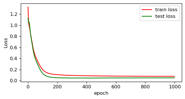
Training the model with the 4 input features with weight decay results in the following plot for the train and test losses. Look that now the test loss does not start increasing as before!
在具有权重衰减的4个输入特征的情况下训练模型,结果显示在下面的火车损失和测试损失图中。 看起来现在测试损失并没有像以前那样开始增加!
It is also important to mention that when you are starting a new project, overfitting is something you should aim for. Start with a model that can overfit the data so that you know that your model has enough ‘flexibility’ to learn the patterns in your data. Then increase regularization, like weight decay, to avoid overfitting!
同样重要的是要提到, 当您开始一个新项目时,过拟合是您应该追求的目标 。 从可以过度拟合数据的模型开始,以便您知道模型具有足够的“灵活性”来学习数据中的模式。 然后增加正则化,例如减重,以避免过度拟合!
家庭作业 (Homework)
I can show you a thousand examples but you will learn more if you can make one or two experiments by yourself! The complete code for these experiments is available on this notebook.
我可以为您展示一千个示例,但是如果您可以自己进行一两个实验,您会学到更多! 在笔记本上可以找到这些实验的完整代码。
- As in the previous lesson, try to play with the learning rate, number of epochs, weight decay and the size of the model. 与上一课一样,尝试发挥学习率,历元数,权重衰减和模型的大小。
- Make experiments and look if the results are what you expected, if not look at the visualizations and try to understand why. 进行实验并查看结果是否符合预期,如果不查看可视化效果并尝试理解原因。
And as always, if you create interesting notebooks with nice animations as a result of your experiments, go ahead and share them on GitHub, Kaggle or write a Medium story!
与往常一样,如果您通过实验创建了带有精美动画的有趣笔记本,请继续在GitHub,Kaggle上分享它们,或撰写一个中型故事!
结束语 (Final remarks)
This ends the second story in the Learn AI Today series!
到此为止,《今日学习AI》系列中的第二个故事结束了!
Please consider joining my mailing list in this link to get updates so that you won’t miss any of the following stories or important updates!
请考虑通过此链接加入我的邮件列表 获取更新,这样您就不会错过以下任何故事或重要更新!
I will also be listing the new stories at learn-ai-today.com, the page I created for this learning journey!
我还将在learning-ai-today.com上列出新故事,该页面是我为这次学习之旅而创建的页面!
And in case you missed it before, this is the link for the Kaggle notebook with the code for this story!
万一您之前错过了它, 这是Kaggle笔记本的链接以及此故事的代码 !
Feel free to give me some feedback in the comments. What did you find most useful or what could be explained better? Let me know!
请随时在评论中给我一些反馈。 您觉得最有用的是什么? 让我知道!
You can read more about my journey on the following stories!
您可以在以下故事中阅读有关我的旅程的更多信息!
Thanks for reading! Have a great day!
谢谢阅读! 祝你有美好的一天!
深度学习分类pytorch


 2336
2336

 被折叠的 条评论
为什么被折叠?
被折叠的 条评论
为什么被折叠?
 到【灌水乐园】发言


