机器学习基础支持向量机svm分类-CSDN博客

本文介绍了SVM分类的基本概念，包括支持向量和超平面。通过一个非线性数据集示例，展示了如何使用SVM进行分类，包括数据预处理、训练模型和评估准确性。还提供了代码实现的步骤，包括数据集导入、划分、特征缩放、模型训练和结果可视化。

摘要生成于 C知道，由 DeepSeek-R1 满血版支持，前往体验 >

In the previous stories, I had given an explanation of the program for implementation of various Regression models. Also, I had described the implementation of the Logistic Regression and the KNN Classification model. In this article, we shall see the algorithm and the implementation of the SVM Classification with a crisp example.

在先前的故事中，我已经解释了用于实现各种回归模型的程序。另外，我已经描述了Logistic回归和KNN分类模型的实现。在本文中，我们将通过一个清晰的示例了解SVM分类的算法和实现。

SVM分类概述 (Overview of SVM Classification)

The Support Vector Machine (SVM) Classification is similar to the SVR that I had explained in my previous story. In SVM, the line that is used to separate the classes is referred to as hyperplane. The data points on either side of the hyperplane that are closest to the hyperplane are called Support Vectors which is used to plot the boundary line.

支持向量机(SVM)分类类似于我在上一个故事中解释的SVR。在SVM中，用于分隔类的线称为hyperplane 。超平面两侧最靠近超平面的数据点称为支持向量 ，用于绘制边界线。

In SVM Classification, the data can be either linear or non-linear. There are different kernels that can be set in an SVM Classifier. For a linear dataset, we can set the kernel as ‘linear’.

在SVM分类中，数据可以是线性的也可以是非线性的。在SVM分类器中可以设置不同的内核。对于线性数据集，我们可以将内核设置为“ 线性 ”。

On the other hand, for a non-linear dataset, there are two kernels, namely ‘rbf’ and ‘polynomial’. In this, the data is mapped to a higher dimension which makes it easier to draw the hyperplane. Afterwards, it is brought down to the lower dimension.

另一方面，对于非线性数据集，有两个内核，即“ rbf ”和“ 多项式 ”。这样，数据被映射到更高的维度，这使得绘制超平面更加容易。之后，将其降低到较低的尺寸。

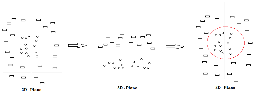
Image for post — SVM Mechanism (Source — Self)

From the above diagram, we can see that there are two classes of shapes, rectangle and circle. As it is difficult to draw a SVM line in the 2D Plane, we map the data points to a higher dimension (3D Plane) and then draw the hyperplane. It is then brought down to the original plane with the SVM Classifier drawn in red color.

从上图可以看出，有两类形状：矩形和圆形。由于很难在2D平面中绘制SVM线，因此我们将数据点映射到更高的维度(3D平面)，然后绘制超平面。然后使用红色绘制的SVM分类器将其放到原始平面。

In this way, the SVM Classifier can be used to classify a data point to which class it belongs from the given dataset. Let us use this algorithm to solve a real-world problem.

这样，SVM分类器可用于对数据点进行分类，该数据点属于给定数据集。让我们使用此算法来解决一个实际问题。

问题分析 (Problem Analysis)

In this implementation of the SVM Classification model, we shall use a Social Network Advertisement dataset which consists of three columns. The first two columns are the independent variables, namely the ‘Age ’and the ‘EstimatedSalary’ and the last column is the dependent variable ‘Purchased’, which is in the binary format denoting whether the individual has bought the product (1) or not (0).

在SVM分类模型的此实现中，我们将使用由三列组成的社交网络广告数据集。前两列是自变量，即“ 年龄”和“ EstimatedSalary” ，最后一列是因变量“ 购买” ，采用二进制格式表示个人是否购买了商品(1)。 (0)。

In this problem, we have to build a SVM Classification model for a company that will classify whether a user of a particular age and with a particular salary will buy their given product or not. Let us now go through the implementation of the model.

在这个问题中，我们必须为公司建立一个SVM分类模型，该模型将对特定年龄和特定薪水的用户是否会购买他们给定的产品进行分类。现在让我们来看一下该模型的实现。

步骤1：导入库 (Step 1: Importing the Libraries)

As always, the first step will always include importing the libraries which are the NumPy, Pandas and the Matplotlib.

与往常一样，第一步将始终包括导入NumPy，Pandas和Matplotlib库。

import numpy as np
import matplotlib.pyplot as plt
import pandas as pd

步骤2：导入数据集 (Step 2: Importing the dataset)

In this step, we shall obtain the dataset from my github repositary which is stored as SocialNetworkAds.csv and store it to the variable dataset. Then we shall assign the corresponding variables to X and Y. Finally, we shall see the first 5 rows of our dataset.

在此步骤中，我们将从我的github存储库中获取数据集，该数据集存储为SocialNetworkAds.csv并将其存储到变量数据集 。然后，我们将相应的变量分配给X和Y。最后，我们将看到数据集的前5行。

dataset = pd.read_csv('https://raw.githubusercontent.com/mk-gurucharan/Classification/master/SocialNetworkAds.csv')X = dataset.iloc[:, [0, 1]].values
y = dataset.iloc[:, 2].valuesdataset.head(5)>>
Age   EstimatedSalary   Purchased
19    19000             0
35    20000             0
26    43000             0
27    57000             0
19    76000             0

步骤3：将资料集分为训练集和测试集 (Step 3: Splitting the dataset into the Training set and Test set)

There are 400 rows in this dataset. We shall split the data into the training and the test set. In this the test_size=0.25 denotes that 25% of the data will be kept as the Test set and the remaining 75% will be used for training as the Training set. Thus, there are about 100 data points in the test set.

该数据集中有400行。我们将数据分为训练和测试集。在这种情况下， test_size=0.25表示将保留25％的数据作为测试集，而将剩余的75 ％的数据用作培训集 。因此，测试集中大约有100个数据点。

from sklearn.model_selection import train_test_split
X_train, X_test, y_train, y_test = train_test_split(X, y, test_size = 0.25)

步骤4：功能缩放 (Step 4: Feature Scaling)

This step of feature scaling is an additional step that can increase the speed of the program as we scale down the values of X to a smaller range. In this, we scale down both the X_trainand the X_test to a small range of -2 to +2. For example, the salary 75000 is scaled down to 0.16418997.

功能缩放的这一步骤是附加步骤，可以在将X的值缩小到较小范围时提高程序的速度。在这种情况下，我们将X_train和X_test到-2到+2的较小范围。例如，薪水75000缩小为0.16418997。

from sklearn.preprocessing import StandardScaler
sc = StandardScaler()
X_train = sc.fit_transform(X_train)
X_test = sc.transform(X_test)

步骤5：在训练集上训练SVM分类模型 (Step 5: Training the SVM Classification model on the Training Set)

Once the training test is ready, we can import the SVM Classification Class and fit the training set to our model. The class SVC is assigined to the variable classifier. The kernel used here is the “rbf” kernel which stands for Radial Basis Function. There are several other kernels such as the linear and the Gaussian kernels which can also be implemented. The classifier.fit() function is then used to train the model.

训练测试准备就绪后，我们可以导入SVM分类类并将训练集拟合到我们的模型中。 SVC类是变量classifier辅助。此处使用的内核是“ rbf”内核，代表径向基函数。还可以实现其他几个内核，例如线性和高斯内核。然后使用classifier.fit()函数来训练模型。

from sklearn.svm import SVC
classifier = SVC(kernel = 'rbf', random_state = 0)
classifier.fit(X_train, y_train)

步骤6：预测测试集结果 (Step 6: Predicting the Test set results)

In this step, the classifier.predict() function is used to predict the values for the Test set and the values are stored to the variable y_pred.

在此步骤中， classifier.predict()函数用于预测测试集的值，并将这些值存储到变量y_pred.

y_pred = classifier.predict(X_test) 
y_pred

步骤7：混淆矩阵和准确性 (Step 7: Confusion Matrix and Accuracy)

This is a step that is mostly used in classification techniques. In this, we see the Accuracy of the trained model and plot the confusion matrix.

这是分类技术中最常用的步骤。在此，我们看到了训练模型的准确性，并绘制了混淆矩阵。

The confusion matrix is a table that is used to show the number of correct and incorrect predictions on a classification problem when the real values of the Test Set are known. It is of the format

混淆矩阵是一个表，用于在已知测试集的实际值时显示有关分类问题的正确和不正确预测的数量。它的格式

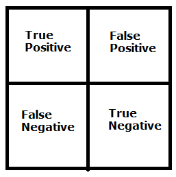
The True values are the number of correct predictions made.

True值是做出正确预测的次数。

from sklearn.metrics import confusion_matrix
cm = confusion_matrix(y_test, y_pred)from sklearn.metrics import accuracy_score 
print ("Accuracy : ", accuracy_score(y_test, y_pred))
cm>>Accuracy :  0.9>>array([[59,  6],
       [ 4, 31]])

From the above confusion matrix, we infer that, out of 100 test set data, 90 were correctly classified and 10 were incorrectly classified, leaving us with an accuracy of 90%.

从上面的混淆矩阵中，我们推断出，在100个测试集数据中，有90个被正确分类，而10个被错误分类，从而使我们的准确性为90％。

步骤8：将实际值与预测值进行比较 (Step 8: Comparing the Real Values with Predicted Values)

In this step, a Pandas DataFrame is created to compare the classified values of both the original Test set (y_test) and the predicted results (y_pred).

在此步骤中，将创建一个Pandas DataFrame来比较原始测试集( y_test )和预测结果( y_pred )的分类值。

df = pd.DataFrame({'Real Values':y_test, 'Predicted Values':y_pred})
df>> 
Real Values   Predicted Values
1             1
0             0
0             0
1             1
0             0
... ...  ... ...
1             1
1             1
0             0
0             0
1             1

This step is an additional step which is not much informative as the Confusion matrix and is mainly used in regression to check the accuracy of the predicted value.

此步骤是一个附加步骤，与Confusion矩阵相比，信息量不多，主要用于回归以检查预测值的准确性。

步骤9：可视化结果 (Step 9: Visualizing the Results)

In this last step, we visualize the results of the SVM Classification model on a graph that is plotted along with the two regions.

在最后一步中，我们在与两个区域一起绘制的图形上可视化SVM分类模型的结果。

from matplotlib.colors import ListedColormap
X_set, y_set = X_test, y_test
X1, X2 = np.meshgrid(np.arange(start = X_set[:, 0].min() - 1, stop = X_set[:, 0].max() + 1, step = 0.01),
                     np.arange(start = X_set[:, 1].min() - 1, stop = X_set[:, 1].max() + 1, step = 0.01))
plt.contourf(X1, X2, classifier.predict(np.array([X1.ravel(), X2.ravel()]).T).reshape(X1.shape),
             alpha = 0.75, cmap = ListedColormap(('red', 'green')))
plt.xlim(X1.min(), X1.max())
plt.ylim(X2.min(), X2.max())
for i, j in enumerate(np.unique(y_set)):
    plt.scatter(X_set[y_set == j, 0], X_set[y_set == j, 1],
                c = ListedColormap(('red', 'green'))(i), label = j)
plt.title('SVM Classification')
plt.xlabel('Age')
plt.ylabel('EstimatedSalary')
plt.legend()
plt.show()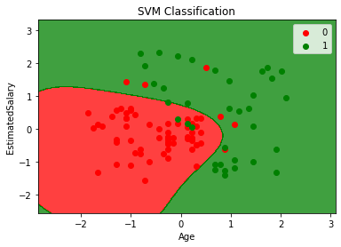

In this plot, There are two regions. The Red region denotes 0, which consists of people who have not bought the product and the Green region denotes 1, which consists of the people who have bought the product. As we have chosen a non-linear kernel (rbf), we are getting regions that are not separated by a linear line.

在该图中，有两个区域。红色区域表示0 ，由尚未购买产品的人组成；绿色区域表示1 ，其由尚未购买产品的人组成。当我们选择了非线性核(rbf)时，我们得到的区域没有被线性线分隔。

If you notice closely, we can see the 10 wrongly classified data points in the test set with the difference in color in the specific region.

如果您密切注意，我们可以看到测试集中的10个错误分类的数据点，其中特定区域的颜色存在差异。

结论— (Conclusion —)

Thus in this story, we have successfully been able to build a SVM Classification Model that is able to predict if a person is going to buy a product based on his age and salary. Do feel free to try out various other common classification datasets that are available on the net.

因此，在这个故事中，我们成功地建立了一个SVM分类模型，该模型能够根据一个人的年龄和薪水来预测他是否打算购买某种产品。请随时尝试网上提供的其他各种常见分类数据集。

I am also attaching the link to my github repository where you can download this Google Colab notebook and the data files for your reference.

我还将链接附加到我的github存储库中，您可以在其中下载此Google Colab笔记本和数据文件以供参考。

You can also find the explanation of the program for other Classification models below:

您还可以在下面找到其他分类模型的程序说明：