


量子属于原子吗
With the advent of Star Wars movie series, we all have started believing that someday, concepts like teleportation, intergalactic travel, etc. will exist. Thinking of teleportation, we remember that during 1980s, a term coined as Quantum Teleportation became very popular, and people started believing that communication can be made possible faster than speed of light someday. So today, let’s discuss the bits and atoms of one of the most fancy technologies of the 21st century “Quantum Computing” and see how much truth is hidden in such science fiction. If this already sounds interesting, then I bet that by the end of this article, you will become familiar with some of the basic terminologies and concepts of Quantum Computing.
随着《 星球大战 》( Star Wars)电影系列的问世,我们所有人都开始相信,总有一天,诸如隐形眼镜,星际旅行等概念将会存在。 考虑到隐形传态,我们记得在1980年代创造了一个术语“ 量子隐形传态”,它变得非常流行,人们开始相信有一天通信的实现速度可能比光速还快。 因此,今天让我们讨论21世纪“量子计算”中最花哨的技术之一的细节,看看这种科幻小说中隐藏了多少真相。 如果听起来很有趣,那么我敢打赌,到本文结尾,您将熟悉一些量子计算的基本术语和概念。
There are a million billion questions in people’s mind, how quantum computing will be beneficial to the world, what shall we get with such a huge investment (yeah building quantum computers are real pain), will it replace classical computers, etc. Google AI Quantum has recently announced that they have demonstrated Quantum Supremacy by completing a task in 200 seconds, which would have taken thousands of years on the most powerful supercomputers in the world today. This was achieved with their most powerful quantum processor, also known as the Sycamore processor, which is comprised of a whooping 54 qubits (“Quantum” bits). So let’s see what quantum computing is, and how do they work.
在人们的头脑中,有一亿亿个问题,量子计算将如何对世界造福,如此巨大的投资我们将获得什么(是的,建造量子计算机是真正的痛苦),它将取代传统计算机,等等。Google AI Quantum最近宣布他们已经证明了量子至上 在200秒内完成一项任务,而在当今世界上最强大的超级计算机上,这将花费数千年。 这是通过其功能最强大的量子处理器(也称为Sycamore处理器)实现的 ,该处理器由多达54个量子比特(“量子”比特)组成。 因此,让我们看看什么是量子计算以及它们如何工作。
The key fundamental difference that separates a quantum computer from a classical computer is the way in which information is stored and processed. A classical computer stores information in the form of bits, which can either be 0 or 1. A quantum computer stores information in the form of a qubit. We won’t discuss how physical qubit systems are made in this article, that is beyond our scope right now. But before telling more about qubits, let’s introduce a bit of mathematics.
将量子计算机与经典计算机区分开来的关键根本区别是信息的存储和处理方式。 经典计算机以位的形式存储信息,可以为0或1。量子计算机以qubit的形式存储信息。 本文不会讨论物理量子位系统的构成方式,这超出了我们的讨论范围。 但是在介绍更多有关量子位之前,让我们先介绍一下数学。
Paul Dirac introduced us the bra-ket notation, which is an easy way of writing vectors. There are two primary states in quantum mechanics, which are called the state |0> and the state |1>. If you don’t get what this weird “|>” thing is, it is just a way of writing column vectors like this
保罗·狄拉克(Paul Dirac)向我们介绍了bra-ket表示法,这是一种编写矢量的简便方法。 量子力学中有两个主要状态,分别称为状态| 0>和状态| 1> 。 如果您不明白这个奇怪的“ |>”是什么,那只是写这样的列向量的一种方式

These vectors are also called orthonormal basis, which means that the magnitude of the vectors is equal to 1, and the dot-product of the two vectors is 0.
这些向量也称为正交基准,这意味着向量的大小等于1,并且两个向量的点积为0。
A set of orthonormal basis vectors describe a new dimension. If there are two orthonormal basis vectors, they describe two dimensions. This means that any two-dimensional vector can be written as a linear combination of the orthonormal basis. As a quick exercise, take any two dimensional vector, like [2 1] (sorry I cannot write it vertically on Medium, but you get that the vector will be vertical ;), and write it as a combination of |0> and |1>. It will look something like a|0> + b|1>, where a and b are two constants. Try to find out the constants. What this means is that, you cannot write one orthonormal basis vector in terms of the other. Then these vectors are called linearly independent. These are also called computational basis states.
一组正交基向量描述了一个新维度。 如果有两个正交基向量,它们将描述两个维度。 这意味着可以将任何二维矢量写为正交法线基础的线性组合 。 作为快速练习,采用任意二维矢量,例如[2 1](对不起,我不能在Medium上垂直书写,但是您会发现矢量将是垂直;),然后将其写为| 0>和|的组合。 1>。 看起来像a | 0> + b | 1>,其中a和b是两个常数。 尝试找出常数。 这意味着,您不能就另一个正交向量编写一个正交向量。 然后将这些向量称为线性独立 。 这些也称为计算基础状态 。
A qubit can be represented in the form
量子位可以用以下形式表示
One thing to notice here is that the constants a and b we are talking about can be real, imaginary or both. (If you are new to imaginary numbers, read here). These are also called complex numbers, numbers which can be imaginary, real or both.
这里要注意的一件事是,我们正在讨论的常数a和b可以是实数,虚数或两者皆可。 (如果您不熟悉虚数,请在此处阅读)。 这些也称为复数 ,可以是虚数,实数或两者皆有的数。
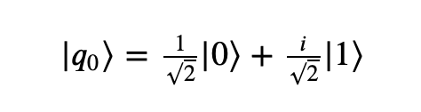
This vector, |q0> is called the qubit’s statevector, it tells us everything we could possibly know about this qubit. For now, we just need to understand that this qubit is neither completely in state |0> nor in state |1>, but a linear combination of both. Such linear combination of orthonormal basis vectors is termed as “superposition”.
这个向量| q0>被称为量子位的状态向量 ,它告诉我们关于这个量子位我们可能知道的一切。 现在,我们只需要了解这个量子位既不是完全处于状态| 0>也不处于状态| 1>,而是两者的线性组合。 正交基向量的这种线性组合被称为“ 叠加 ”。
Let’s introduce one more term, “amplitude”. Amplitude denotes the coefficient before the orthonormal basis vectors that we use to write our statevector. So, for the general case a|0> + b|1>, a is the amplitude of |0> state, whereas b is the amplitude of |1> state.
让我们再介绍一个术语“ 振幅 ”。 振幅表示我们用来编写状态向量的正交基向量之前的系数。 因此,对于一般情况a | 0> + b | 1>,a是| 0>状态的幅度,而b是| 1>状态的幅度。
There is also a constraint associated with the amplitudes of the statevector. The “sum of square of modulus of amplitudes of a statevector should be equal to 1”. I know there’s a lot to unpack in this statement, but what it basically means is that
还存在与状态向量的幅度相关联的约束。 “状态向量的振幅模量的平方和应等于1” 。 我知道此语句中有很多要解压的内容,但基本上意味着
|a|²+|b|²=1, as simple as it can get.
| a |²+ | b |²= 1,尽可能简单。
This is called “normalzation”, and it basically means that the “every vector must have unit length”.
这称为“ 归一化 ”,它的基本含义是“ 每个向量都必须具有单位长度”。
So a brief summary till now. We have introduced “kets” as a new notation to represent vectors. We have seen how any vector can be represented as a linear combination of orthonormal basis vector states, the representation being called a “statevector”, and the term used to describe this phenomenon is called “superposition”. We have also seen the “normalization” constraint, which limits the length of every vector defined to unity.
到目前为止,还是一个简短的摘要。 我们引入了“ kets”作为表示矢量的新符号。 我们已经看到如何将任何矢量表示为正交基矢量状态的线性组合,该表示称为“状态矢量”,而用于描述该现象的术语称为“ 叠加”。 我们还看到了“ 归一化”约束,该约束将每个矢量的长度限制为1。
Phew!!! That was a lot of maths. So let’s do some hands-on coding with IBM Qiskit. Qiskit is IBM’s open source SDK for working with quantum computers at the level of pulses, circuits and algorithms. Qiskit accelerates the development of quantum applications by providing the complete set of tools needed for interacting with quantum systems and simulators. If you want to install Qiskit, check all the various options for installing and running Qiskit here.
ew! 那是很多数学。 因此,让我们使用IBM Qiskit进行一些动手编码。 Qiskit是IBM的开源SDK,用于在脉冲,电路和算法级别与量子计算机一起工作。 Qiskit通过提供与量子系统和仿真器进行交互所需的整套工具,加速了量子应用程序的开发。 如果要安装Qiskit,请在此处检查安装和运行Qiskit的所有各种选项。
Open up Jupyter notebook on your PC. To run a cell, press Shift+Enter. In the first cell, type the following. These will import all the necessary tools required for this lab exercise.
在PC上打开Jupyter笔记本。 要运行单元格,请按Shift + Enter。 在第一个单元格中,键入以下内容。 这些将导入此实验练习所需的所有必要工具。
from qiskit import QuantumCircuit, execute, Aer
from qiskit.visualization import plot_histogram, plot_bloch_vector
from math import sqrt, pi
We will use QuantumCircuit to create a new circuit. We generally pass two numbers to it, first one represents the number of qubits we need in our circuit, and second one is the number of “classical” bits to take measurement (we will come to what is measurement later). For now, we will just initialise our circuit with just one qubit as follows
我们将使用QuantumCircuit创建一个新电路。 我们通常将两个数字传递给它,第一个数字代表我们电路中所需的qubit数量,第二个数字是进行测量的“经典”位数(我们将在后面介绍测量)。 现在,我们将仅用一个量子位来初始化电路,如下所示
qc = QuantumCircuit(1) # Create a quantum circuit with one qubitRemember that just as we initialise our Quantum Circuit, the qubits start in the state |0>. This is just a default to make further calculations easier. But Qiskit provides us the flexibility to initialise our qubits with any numbers we want. This can be done using the initialize() method. We pass a list of numbers and tell which qubit we want to initialise. List is a python data structure.
记住,当我们初始化量子电路时,量子位以| 0>状态开始。 这只是默认设置,可以使进一步的计算更加容易。 但是Qiskit为我们提供了使用所需的任何数字初始化qubit的灵活性。 这可以使用initialize()方法完成。 我们传递一个数字列表 ,并告诉我们要初始化哪个量子位。 List是python数据结构。
Important: The list of numbers you pass as an argument to initialize() method should follow the “Normalization” rule.
重要提示:您作为initialize()方法的参数传递的数字列表应遵循“ 规范化”规则。
Okay, in the next cell, we initialize our qubit to the |1> state in the following way
好的,在下一个单元格中,我们按照以下方式将qubit初始化为| 1>状态
qc = QuantumCircuit(1)  # Create a quantum circuit with one qubit
initial_state = [0,1]   # Define initial_state as |1>
qc.initialize(initial_state, 0) # Apply initialisation operation to the 0th qubit
qc.draw('text')  # Let's view our circuit (text drawing is required for the 'Initialize' gate due to a known bug in qiskit)
If you initialize your qubit that does not follow the normalization rule, something like this
如果您初始化不遵循规范化规则的qubit,则类似以下内容
vector = [1,1]
qc.initialize(vector, 0)
You will get an error on running this cell as
您将在运行此单元格时收到错误消息
QiskitError                               Traceback (most recent call last)
<ipython-input-12-ddc73828b990> in <module>      1 vector = [1,1]
----> 2 qc.initialize(vector, 0)
/usr/local/anaconda3/lib/python3.7/site-packages/qiskit/extensions/quantum_initializer/initializer.py in initialize(self, params, qubits)    252     if not isinstance(qubits, list):    253         qubits = [qubits]
--> 254     return self.append(Initialize(params), qubits)    255     256
/usr/local/anaconda3/lib/python3.7/site-packages/qiskit/extensions/quantum_initializer/initializer.py in __init__(self, params)     56         if not math.isclose(sum(np.absolute(params) ** 2), 1.0,     57                             abs_tol=_EPS):
---> 58             raise QiskitError("Sum of amplitudes-squared does not equal one.")     59      60         num_qubits = int(num_qubits)
QiskitError: 'Sum of amplitudes-squared does not equal one.
To get the resulting statevector after performing such an operation of a qubit, we will use Qiskit’s “statevector_simulator”. There are other simulators as well, but more on that later.
为了在执行了qubit运算之后获得结果状态向量,我们将使用Qiskit的“ statevector_simulator”。 也有其他模拟器,但稍后会介绍更多。
backend = Aer.get_backend('statevector_simulator') # Tell Qiskit how to simulate our circuitThen we will use execute to run our circuit, and the .result() to get our required statevector.
然后,我们将使用execute运行电路,并使用.result ()获得所需的状态向量。
qc = QuantumCircuit(1) # Create a quantum circuit with one qubit
initial_state = [0,1]   # Define initial_state as |1>
qc.initialize(initial_state, 0) # Apply initialisation operation to the 0th qubit
result = execute(qc,backend).result() # Do the simulation, returning the result
from result, we can then get the final statevector using .get_statevector()
从result ,我们可以使用.get_statevector()获得最终的状态.get_statevector()
qc = QuantumCircuit(1) # Create a quantum circuit with one qubit
initial_state = [0,1]   # Define initial_state as |1>
qc.initialize(initial_state, 0) # Apply initialisation operation to the 0th qubit
result = execute(qc,backend).result() # Do the simulation, returning the result
out_state = result.get_statevector()
print(out_state) # Display the output state vector[0.+0.j 1.+0.j]
Note that j here is used to represent imaginary numbers.
注意,这里的j用于表示虚数。
Congratulations on implementing your first quantum circuit. Although it is of not much importance, but we have built our fundamental quantum circuit. We will build upon this as the blog series will continue.
恭喜您实现了第一个量子电路。 尽管它并不是很重要,但是我们已经建立了基本的量子电路。 随着博客系列的继续,我们将以此为基础。
We are left with one last concept in this article, which is “measurement”.
本文只剩下最后一个概念,即“ 测量”。
Before speaking anything about measurement, let me introduce you a small topic, called the “inner product”. This is a generalisation of the vector dot product. We use the inner product between a bra-(row-vector) and a ket-(column vector) like this
在谈论有关测量的任何内容之前,我先介绍一个小话题,称为“ 内部产品 ”。 这是向量点积的概括。 我们使用bra-(行向量)和ket-(列向量)之间的内积
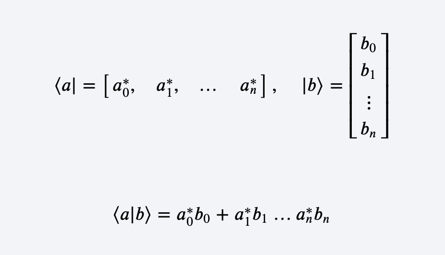
The asterisk(*) above a number denotes “complex conjugate” of that number. If a complex number is written as a+jb, its complex conjugate will be a-jb.
数字上方的星号(*)表示该数字的“ 复共轭” 。 如果复数写为a + jb ,则其复共轭将为a-jb。
A very important rule for measurement
一个非常重要的测量规则

If you brush up a little maths of linear algebra, then you will realise that if we write any quantum state as |x> = a|0> + b|1>, then the probability of measuring state |x> as |0> is |a|², and that of |1> is |b|². Try to do this by taking |x> as |0> and |1>, and ⍦ as some “a|0> + b|1>”.
如果您复习一下线性代数的一些数学知识,那么您将认识到,如果我们将任何量子态写为| x> = a | 0> + b | 1>,那么测量状态| x>的概率为| 0>是| a |²,而| 1>的| b |²。 尝试将| x>设为| 0>和| 1>,将⍦设为“ a | 0> + b | 1>”。
Wait, we just found out the famous Born rule. It says that the probability of finding a quantum state in another given quantum state is just the square of modulus of inner product of the two states.
等等,我们才发现了著名的天生法则 。 它说在另一个给定的量子态中找到一个量子态的概率只是这两个态的内积模数的平方。
Let’s check this using Qiskit’s statevector_simulator. First we will initialise our qubit like this
让我们使用Qiskit的statevector_simulator进行检查。 首先,我们将像这样初始化我们的量子比特
qc = QuantumCircuit(1) # Redefine qc
initial_state = [0.+1.j/sqrt(2),1/sqrt(2)+0.j]
qc.initialize(initial_state, 0)
qc.draw('mpl')
This should initialize our qubit as
这应该将我们的量子位初始化为

To verify this, let’s use our statevector_simulator.
为了验证这一点,让我们使用statevector_simulator。
state = execute(qc, backend).result().get_statevector()
print("Qubit State = " + str(state))
Finally, let’s measure this qubit
最后,让我们测量这个量子位
qc.measure_all()
qc.draw('mpl')
Now, let’s simulate the circuit and get our measured state
现在,让我们模拟电路并获得我们的测量状态
state = execute(qc, backend).result().get_statevector()
print("State of Measured Qubit = " + str(state))
You will always get result as
您将始终获得如下结果
State of Measured Qubit = [0.+0.j 1.+0.j]#ORState of Measured Qubit = [1.+0.j 0.+0.j]Phew!!!!! That was a lot to take in one article. Today we have seen terms like “qubit”, “state-vectors”, “superposition”, “normalisation”, “Born Rule” and many more. These are all just the fundamentals of quantum computing. There are many more fundamentals, but we shall cover them in the next article. I’ve tried to simplify concepts as much as possible. Also, check out the links that I’ve attached with this article, they are super useful and will give you a complete picture about what I’m referring to.
ew !!!!! 一篇文章要花很多钱。 今天,我们已经看到了诸如“量子位”,“状态向量”,“叠加”,“归一化”,“出生规则”之类的术语。 这些全都是量子计算的基础。 还有更多基础知识,但是我们将在下一篇文章中介绍。 我试图尽可能简化概念。 另外,请查看本文附带的链接,它们非常有用,它们将为您提供有关我所指的内容的完整图片。
PSST: Most of my work here is inspired from Qiskit’s community textbook, which is an awesome resource to learn from. If you want to check that out, it is linked here. You can give it a read, or maybe download the Jupyter notebook and run on your local machine. Both works fine. One additional thing that’s mentioned there is about the Bloch Sphere, and I could have mentioned that here also. But it would be a lot to take in this article. I will do it in the next article, along with some cool stuff like Quantum Teleportation.
PSST :我在这里所做的大部分工作都来自Qiskit的社区教科书 ,这是一个很棒的学习资源。 如果您想查看,请在此处链接。 您可以阅读它,或者下载Jupyter笔记本并在本地计算机上运行。 两者都很好。 这里提到的另一件事是关于Bloch Sphere的 ,我也可以在这里提到。 但是这篇文章要花很多时间。 我将在下一篇文章中进行介绍,同时还会介绍一些很酷的东西,例如Quantum Teleportation。
So it is still not clear to us whether communication can be done faster than speed of light. Just to break the ice, I will say the answer here. But that shouldn’t stop you guys from reading the next article on Quantum Teleportation, as it will discuss the process in details.
因此,我们仍然不清楚通讯是否可以比光速快。 只是为了打破僵局,我在这里说答案。 但这并不能阻止你们阅读下一篇有关量子隐形传态的文章,因为它将详细讨论该过程。
Till then, happy Quantum Computing.
到那时,快乐的量子计算。
Oh yeah, I forgot!!! We cannot communicate faster than speed of light. The Theory of Relativity formulated by Einstein is still very true even in the 21st century.
哦,是的,我忘了!!! 我们交流的速度不能超过光速。 即使在21世纪,爱因斯坦提出的相对论仍然非常正确。
翻译自: https://medium.com/quantumcomputingindia/the-bits-and-atoms-of-quantum-computing-bcd580e61257
量子属于原子吗


 718
718

 被折叠的 条评论
为什么被折叠?
被折叠的 条评论
为什么被折叠?
 到【灌水乐园】发言


