机器学习之梯度与梯度下降法_了解机器学习梯度下降的基本概念

机器学习之梯度与梯度下降法

Gradient Descent is one of the most commonly used algorithms in Machine Learning, in this article we will work through the complexity and try to make it understandable for everyone.

梯度下降是机器学习中最常用的算法之一，在本文中，我们将研究复杂性并尝试使每个人都能理解它。

1. Introduction to Gradient Descent

   梯度下降简介

Simply put, Gradient Descent is an algorithm which aims to find the optimal points in a distribution, normaly with prediction purposes. For exemple, let’s imagine that we want to find a way to accurrately predict the property prices of a residential area in the vicinity of Barcelona. We are given a scatter plot (shown below) that holds the values of price and square metres of properties recently sold in the area. The x-axis holds the total square metre values, and the y-axis, their corresponding price. Hence, each dot represents a property with a determinated price and square foots.

简而言之， 梯度下降法是一种旨在发现分布中的最佳点的算法，通常具有预测目的。 例如，让我们想象一下，我们想找到一种方法来准确预测巴塞罗那附近住宅区的房价。 我们得到了一个散点图(如下所示)，该散点图包含该区域最近出售的房地产的价格和平方米的值。 x轴保存平方米总值，y轴保存相应的价格。 因此，每个点代表具有确定价格和平方英尺的属性。

What can the Gradient Descent algorithm help us out with in this context ?

在这种情况下， 梯度下降算法可以为我们提供什么帮助？

What Gradient Descent is set to do, is find the best fitting line between the dots, also known as linear regression model, the model will express the linear relationship between Square Metres and Price, and hopefully would help us predict the market price for future properties on the market.

G 辐射下降的设置是找到点之间的最佳拟合线，也称为线性回归模型，该模型将表达平方米与价格之间的线性关系，并希望能帮助我们预测未来的市场价格市场上的房地产。

To explain the Gradient Descent Algorithm we will start by drawing a randomly positioned line in our graph. And we comes up with this:

为了解释梯度下降算法，我们将从在图形中绘制一条随机放置的线开始。 我们想出了这个：

2. Seeking the best Error Measurement

2.寻求最佳的误差测量

Now will have to give the algorithm some mathematical error measurement so he knows how badly he has performed, how far away he is from the optimal point and what steps to take to get there on. However, prior to doing that, we’ll have to teach the algorithm something even more basic, that is, what a linear function looks like mathematicly.

现在必须给该算法进行一些数学上的误差测量，以便他知道自己的执行情况有多差，距最佳点有多远以及到达该点要采取什么步骤。 但是，在此之前，我们必须向算法讲些更基础的东西，即线性函数在数学上看起来是什么样的。

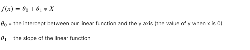
Now the machine knows that a linear function is made up of two parameters that he can tweak to get different linear functions.

现在，机器知道线性函数由两个参数组成，他可以调整这些参数以获得不同的线性函数。

Next, we have to think about the error measure we are going to train the algorithm with. Our optimal line should be the one that minimizes the distance between the line drawn and the given points in our graph, that is, the linear function that furthest diminishes the difference between the actual prices and the predicted ones for all given square metre levels. In the mathematical language would look like this:

接下来，我们必须考虑将要用来训练算法的错误度量。 我们的最佳线应该是使绘制的线与图形中给定点之间的距离最小的线，即，对于所有给定的平方米水平，最远的线性函数会减小实际价格与预测价格之间的差异。 在数学语言中将如下所示：

Therefore, what the above mathematical expression says is: look for a function f(x) that minimizes the sum of the residuals (actual minus predicted values). To be more mathematically precise we should’ve said that the function looks to minimize f(theta_0, theta_1), the thetas are the parameters that change our predicted y, therefore, our final error mesurement. But hold on a second, the function above doesn’t quite add-up, because let’s say we have a pair of predictions, the first one misses the actual price by +50,000 €, and second one falls short by -50,000 €, then, if we go ahead and calculate the error by adding up the two prediction errors, we would get 0, the algorithm would wrongly regard it as a perfect model. To prevent this from happening, we are going to tweak our error measurement equation a bit, and come up with a modified version that goes by the fancy name of the mean squared error (MSE). Here you have it:

因此，以上数学表达式表示的是：寻找一个使残差之和(实际减去预测值)最小的函数f(x )。 为了更精确的数学，我们应该已经表示，该功能看起来尽量减少F(theta_0，theta_1)，该θ驱动是改变我们的预测的y，因此，我们最终的误差测宽的参数。 但是请稍等，上面的函数并没有完全相加，因为我们有一对预测，第一个预测比实际价格少了+50,000€，第二个则差了-50,000€，然后，如果我们继续将两个预测误差相加来计算误差，我们将得到0，该算法会错误地将其视为理想模型。 为了防止这种情况的发生，我们将稍微调整误差测量公式，并提出一个修改后的版本，该版本带有均方误差(MSE)的奇特名称。 在这里，您拥有它：

The m term you see added to the equation stands for the number of instances (dots) that we are going to compute, it is multiplied by the other part of the equation to get the mean value.

您在方程式中看到的m项代表我们要计算的实例数(点)，将其乘以方程式的其他部分即可得到平均值。

So, to recap, we are are telling the algorithm we want a linear function that minimizes the mean squared error, wich is a measure that computes the difference between predicted and actual values, so we want that difference to be as small as it can possibly be given a linear model.

因此，回顾一下，我们正在告诉算法，我们需要一个线性函数以最小化均方误差，这是一种计算预测值与实际值之间的差异的量度，因此我们希望该差异尽可能小给出线性模型。

3. Teaching Gradient Descent

3.教学梯度下降

Finally, we have to teach the algorithm how to navegate the graph looking for the optimal regression line. Well go about this task by first asking him to computing different values for both, the intercept and the slope (components of linear function) and evaluate the their mean squared errors. The graph below shows an exemple of what we’re trying to come up with.

最后，我们必须教算法如何导航图以寻找最佳回归线。 首先，请他为截距和斜率(线性函数的分量)计算不同的值，然后评估它们的均方误差 ，以完成此任务。 下图显示了我们要提出的示例。

https://www.ritchieng.com/one-variable-linear-regression/ https://www.ritchieng.com/one-variable-linear-regression/

Notice that what we have here is a three dimentional graph, where the vertical axis represents the error term (mean squared error) for every pair of values in the linear model (intercept — theta zero, and slope — theta 1).

请注意，这里有一个三维图，其中垂直轴代表线性模型中每对值对的误差项( 均方误差) (截距-theta零和斜率-theta 1)。

Therefore, we want to find a line that minimizes that error, differently put, we are looking a combination of parameters (interecept and slope) that bring the error term (graph vertical axis) down to the lowest possible point (minimum). For those of you who know a bit about algebra, a bell must have rung in your head, what we need here is to derivate the equation and solve for the pair of parameters that make the derivative equal to 0, that would be the lowest point in our graph, hence our two parameters for the best fitting line, Gradient Descent does exactly that.

因此，我们想找到一条使误差最小化的线，换句话说，我们正在寻找参数(截距和斜率)的组合，这些参数使误差项(图形垂直轴)下降到最低点(最小)。 对于那些对代数有所了解的人，钟声一定在您的脑海中，我们这里需要的是推导等式并求解使导数等于0的一对参数，这将是最低点在我们的曲线图中，因此有两个参数是最佳拟合线， Gradient Descent正是这样做的。

4. Intuition

4.直觉

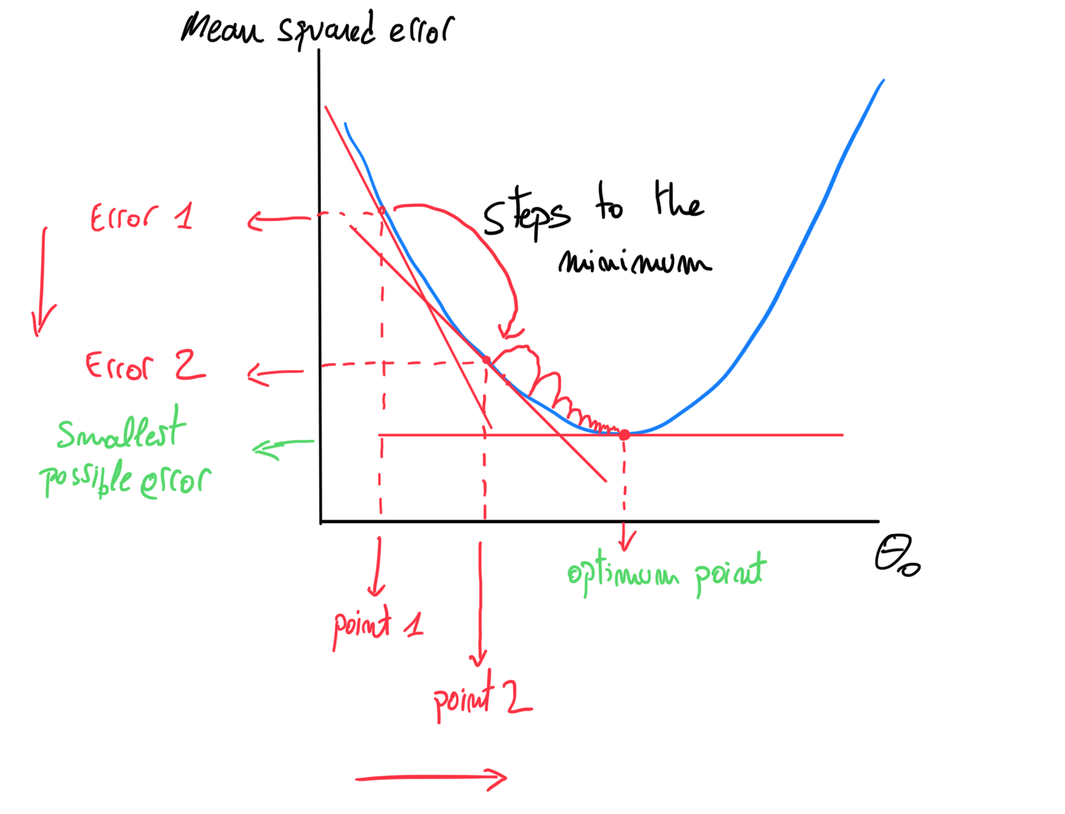
The graph below shows fundamentally the same as the 3-D graph plotted earlier, but looked at only from the theta_0’s perspective, in other words we simplified the graph by omitting one of the axis (theta_1).

下面的图基本上与之前绘制的3-D图相同，但是仅从theta_0的角度看，换句话说，我们通过省略其中一个轴( theta_1)简化了该图。

The red tangent in the graph represents the derivative of the point our machine chose to start from, in our search for the best fitting line. We want the algorithm to find out the derivative that equals 0, it would be represented as a flat tangent in our error function.

图中的红色切线表示我们的机器在寻找最佳拟合线时选择开始的点的导数。 我们希望算法找出等于0的导数，在我们的误差函数中将其表示为平切线。

What Gradient Descent does is, through an array of iterations (steps), goes progressively down the error function approaching its minimim point, when it finally attains it, the algorithm understand it has converged to the optimum solution, and stops. As you can, hopefully, appreciate in the graph below, the steps shorten as the minimum is approach, we’ll get into why that is when we explain the mathematical logic behind Gradient Descent .

梯度下降的作用是通过一系列迭代(步骤)逐步降低误差函数，使其接近最小点，当最终达到该点时，算法将其理解为已收敛至最佳解，然后停止。 如您所愿，希望您能在下图中看到，步骤越短越好，步骤越短，在解释Gradient Descent背后的数学逻辑时，我们将了解为什么。

It is important to bear in mind that this way-to-the-minimum process is carried out by both theta_0 and theta_1 concurrently, meaning the next point in our graph is influenced by both, the step in theta_0 and theta_1, even though the later is not depicted above, you have to imagine a graph where the algorithm is figuring its way down to the minimum but, this time, for theta_1.

重要的是要记住，这种最小化方法是同时由theta_0和theta_1进行的，这意味着图形中的下一个点受theta_0和theta_1中的步长影响，即使稍后上面没有描述，您必须想象一个图形，其中算法正在将其方法降至最小，但是这次是theta_1 。

5. A bit of maths…

5.一点数学…

Understand that we are being a bit sploppy, mathematically speaking, in an effort to do away with complex mathematical notation.

请理解，从数学上讲，我们正在变得有点杂乱，以消除复杂的数学符号。

Let’s go through the components of the formula below from right to left. First, we have the derivative of both thetas with respect to the mean squared error (vertical axis in our 3D graph), that is simply the derivatives we have drawn as tangents in our graph above. Note that in our graph those derivatives are negative (negative slope), and they are flattened (less negative) as they approach the minimum. The next term we have is the Learning Rate in blue, this is simply the step size of our Gradient Descent. And by multiplying those two terms and substracting the result from the last theta’s values, we get the new thetas, with wich we will repeat the steps.

让我们从右到左浏览以下公式的组成部分。 首先，相对于均方误差 (我们的3D图形中的垂直轴)，我们拥有两个theta 的导数，也就是我们在上述图形中作为切线绘制的导数。 请注意，在我们的图中，这些导数为负(负斜率)，并且在逼近最小值时变平(负的负值)。 下一个术语是蓝色的学习率 ，这只是我们的梯度下降步长。 而由这两个方面相乘并从其减去从上次THETA的值的结果，我们得到了新的θ驱动，具有至极我们将重复上述步骤。

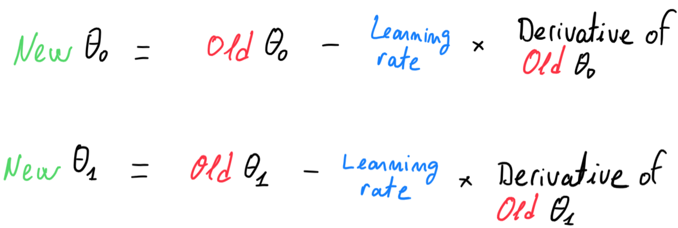
Note that this make sence because if, like in our case, our derivative of theta_0 starting point is negative, let’s say -8, by multiplying it by a learning rate of 0.1, we get -0.8, which once substracted by the prior theta value, makes it increment (two negative turn into positive) wich will result in an advance in theta, nudged towards the right hand site of our graph, precisally where our minimum value lays (exactlly what happened in our graph).

请注意，这是因为如果像我们的情况一样， theta_0起点的导数为负，比方说-8，将其乘以0.1的学习率，则得到-0.8 ，一旦将其减去先前的theta值，使其递增 (由两个负值变为正值)将导致theta向前移动，向我们图的右手侧移动，恰好是我们的最小值所处的位置(恰好是我们图中发生的情况)。

On our second iteration, the slope would have been diminished, let’s say to -5, therefore when multiplied again by the learning rate 0.1, equals -0.5, hence 0.5 to be added to our latest theta value, resulting in a smaller step that the prior one (0.8), and the next step will be one more time smaller than the later, and so on. This is the logic why our steps are increaingly smaller every time Gradient Descent advances along the error function and toward the optimum point.

在我们的第二次迭代中，斜率将减小，例如为-5，因此当再次乘以学习率0.1时，其斜率将等于-0.5，因此将0.5添加到我们的最新theta值中，从而导致该步长较小前一个(0.8)，而下一步骤将比后一个步骤小一倍，依此类推。 这就是为什么每次梯度下降沿误差函数并达到最佳点时我们的步伐越来越小的逻辑。

6. Applying Gradient Descent to our data

6.将梯度下降应用于我们的数据

Now that we have a grasp on the logic the algorithm follows. Let’s apply the Gradient Descent Algorithm to the data of property prices in Barcelona we started with, and see how it does.

现在我们已经掌握了算法遵循的逻辑。 让我们将梯度下降算法应用于我们刚开始的巴塞罗那的房地产价格数据，看看它是如何实现的。

Voilà, exactly as expected! The algorithm started by drawing a random line in the plain (bottom line) and through an array of iterations, in which the two parameters of the line (theta0 and theta1) are constandly tweaked, the algorithm finally gets to the best fitting line, which at the same time equals the minimum possible mean squared error (our error mesurament) in the graph (the minimum point in the 3D graph).

Voilà，完全符合预期！ 该算法首先在普通线(底部线)中绘制一条随机线，然后通过一系列迭代，其中始终对线的两个参数(theta0和theta1)进行调整，算法最终达到最佳拟合线，即同时等于图(3D图中的最小点)中的最小均方误差(我们的误差度量)。

翻译自: https://medium.com/@pauor96/understanding-basic-concepts-of-machine-learning-gradient-descent-7c50aaacc46c

机器学习之梯度与梯度下降法