信封加密 数据秘钥_信封背面快速数据分析

信封加密 数据秘钥

内部AI(Inside AI)

Data analysis is a vital element of any machine learning workflow. The performance and accuracy of any machine learning model prediction hinge on the data analysis and follow-on appropriate data preprocessing. Every machine learning professional should be adept in data analysis.

数据分析是任何机器学习工作流程的重要组成部分。 任何机器学习模型预测的性能和准确性都取决于数据分析和后续适当的数据预处理。 每位机器学习专业人员都应该擅长数据分析。

In this article, I will discuss four very quick data visualisation techniques which can be achieved with few lines of code and can help to plan the data pre-processing required.

在本文中，我将讨论四种非常快速的数据可视化技术，这些技术可以用几行代码实现，并且可以帮助计划所需的数据预处理。

We will be using Indian Liver Patient Dataset from the open ML to learn quick and efficient data visualisation techniques. This data set contains a mix of categorical and numerical independent features and diagnosis result as the liver and non-liver condition.

我们将使用开放式ML中的印度肝病患者数据集来学习快速有效的数据可视化技术。 该数据集包含分类和数值独立特征以及肝脏和非肝脏疾病的诊断结果。

from sklearn.datasets import fetch_openml
import pandas as pd
import matplotlib.pyplot as plt
import seaborn as sns

I feel it is easier and efficient to work with Pandas dataframe than default bunch object. The parameters “as_frame=True” ensures that the data is a pandas DataFrame, including columns with appropriate data types.

我觉得使用Pandas数据框比默认的束对象更容易，更有效。 参数“ as_frame = True”确保数据是pandas DataFrame，包括具有适当数据类型的列。

X,y= fetch_openml(name="ilpd",return_X_y=True,as_frame=True)
print(X.info())

As the independent data is in Pandas, we can view the number of features, the number of records with null values, and data type of each feature with “info”.

由于独立数据在Pandas中，因此我们可以使用“ info”查看要素数量，具有空值的记录数以及每个要素的数据类型。

Independent features, count and datatypes — based on the above code discussed (image by author)

独立的功能，数量和数据类型-基于以上讨论的代码(作者提供的图片)

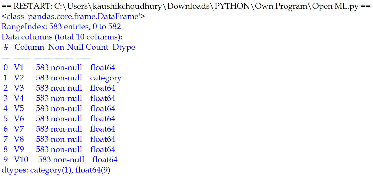
It immediately provides a lot of information about the independent variables with just one line of code.

它仅用一行代码即可立即提供有关自变量的大量信息。

Considering, we have several numerical features it is prudent to understand the correlation among these variables. In the below code, we have created a new dataframe X_Numerical without the categorical variable “V2”.

考虑到我们有几个数值特征，谨慎地理解这些变量之间的相关性是很谨慎的。 在下面的代码中，我们创建了一个没有分类变量“ V2”的新数据框X_Numerical。

X_Numerical=X.drop(["V2"], axis=1)

Few of the machine learning algorithm doesn’t perform well with highly linearly related independent variables. Also, the objective is always to build a machine learning model with the minimum required variables/dimensions.

在高度线性相关的自变量中，很少有机器学习算法不能很好地执行。 同样，目标始终是建立具有最小所需变量/尺寸的机器学习模型。

We can get the correlation among all the numerical features using the “corr” function in Pandas.

我们可以使用Pandas中的“ corr”函数获得所有数值特征之间的相关性。

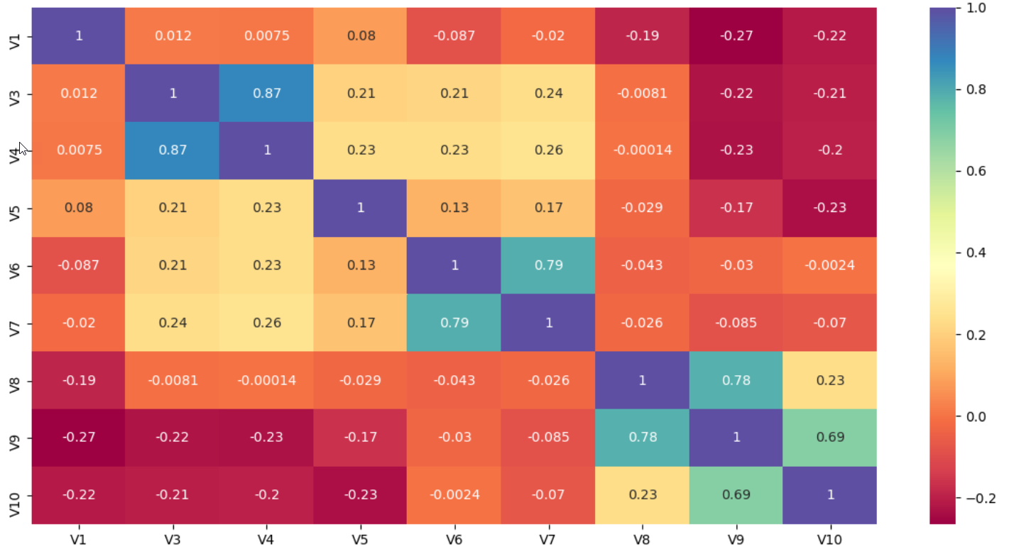
With the seaborn package, we can plot the heatmap of the correlation to get a very quick visual snapshot of the correlation among the independent variables.

使用seaborn软件包，我们可以绘制相关性的热图，以快速获得独立变量之间相关性的直观快照。

relation=X_Numerical.corr(method='pearson')
sns.heatmap(relation, annot=True,cmap="Spectral")
plt.show()

In a glance, we can conclude that the independent variable V4 and V3 have close relation and few of the features like V1 and V10 are loosely negatively correlated.

乍一看，我们可以得出结论：自变量V4和V3具有密切的关系，并且很少有像V1和V10这样的特征是负相关的。

Correlation matrix of independent features based on the above code discussed (image by author)

基于以上讨论的代码，独立特征的相关矩阵(作者提供的图片)

After knowing the correlation among the features next, it will be useful to get a quick sense of the distribution of values for numerical features.

接下来了解了特征之间的相关性之后，快速了解数字特征的值的分布将很有用。

Just like the correlation function, Pandas a native function ‘hist’ to get the distribution of the features.

就像相关函数一样，Pandas使用本机函数“ hist”来获取特征的分布。

X_Numerical.hist(color="Lightgreen")
plt.show()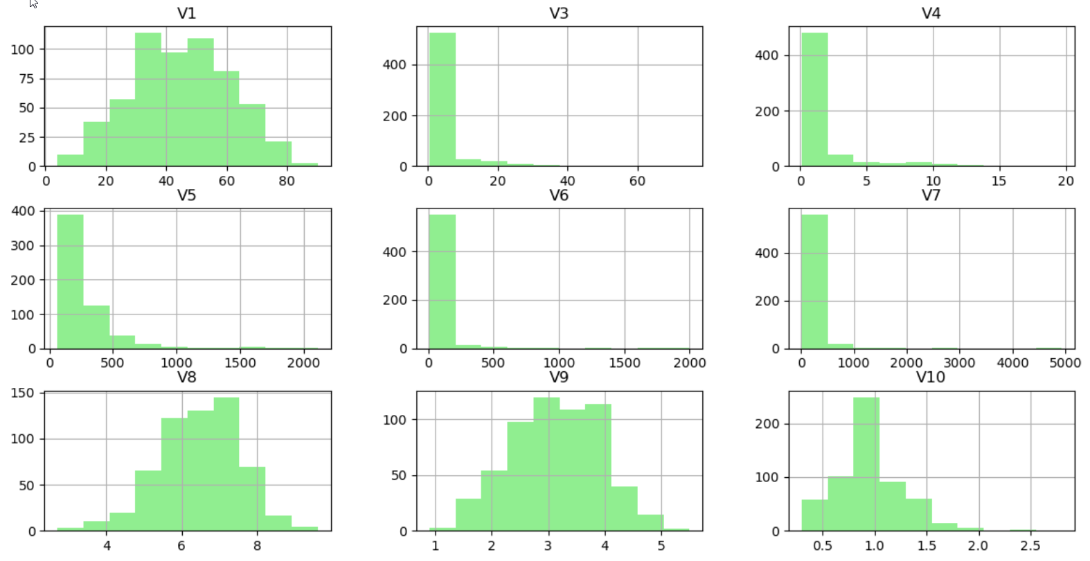

Distribution of independent features based on the above code discussed (image by author)

根据上面讨论的代码分配独立功能(作者提供图片)

Until now the power and versatility of pandas are clearly illustrated. We could get the relation among numerical features and distribution of the features with only two lines of code.

到目前为止，熊猫的力量和多功能性都得到了清晰的说明。 我们只需两行代码就可以得到数值特征和特征分布之间的关系。

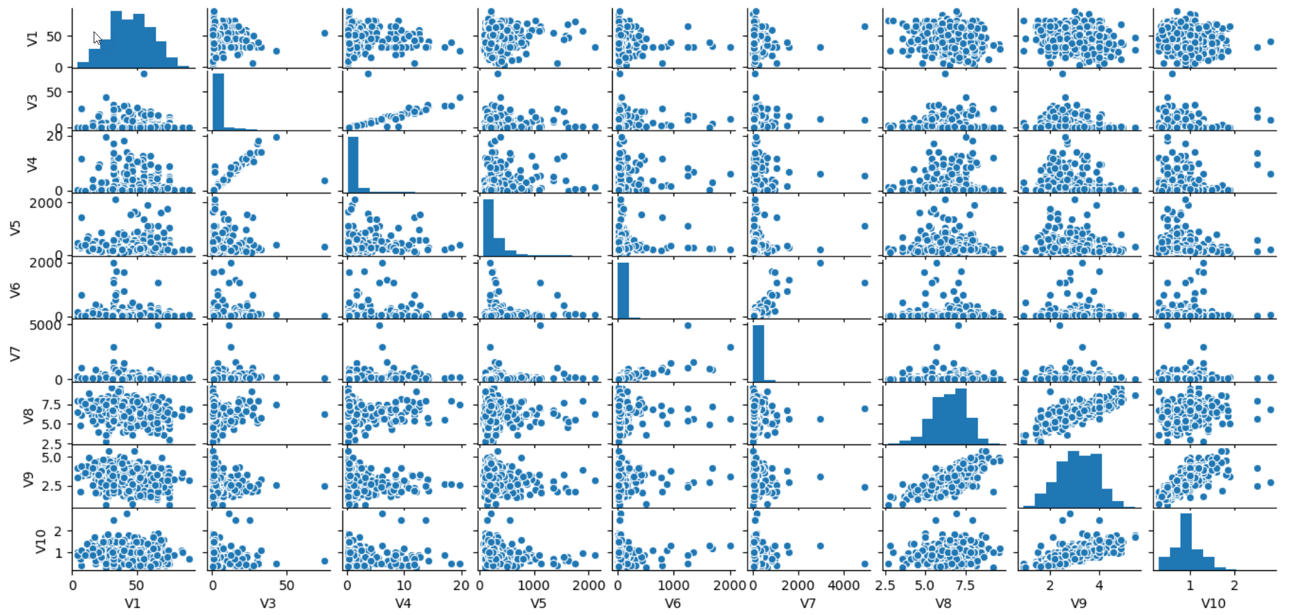
Next, it will be interesting to get a better sense of the numerical independent variables with scatter plots between all the numerical variable combinations.

接下来，通过所有数值变量组合之间的散点图更好地理解数值自变量是很有意思的。

sns.pairplot(X_Numerical)
plt.show()

We can identify the variables which are positively or negatively related with the help of visualisation. Also, with a glance, the features which have no relation among themselves can be identified.

我们可以借助可视化来确定正相关或负相关的变量。 而且，一眼就能识别出彼此之间没有关系的特征。

Scatter plot of independent features based on the above code discussed (image by author)

根据以上讨论的代码，独立特征的散点图(作者提供的图像)

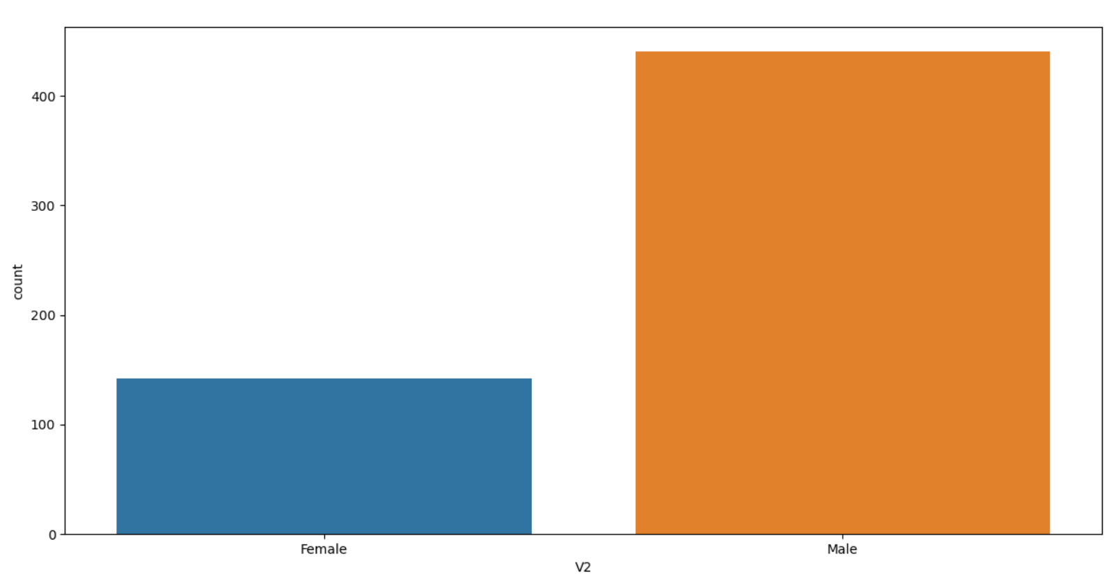
Finally, we can learn about the distribution of the categorical feature with the count plot.

最后，我们可以通过计数图了解分类特征的分布。

sns.countplot(x="V2", data=X)
plt.show()

We get to know that males are over-represented in the dataset compare to females. It is vital to understand if we have an imbalanced dataset and take appropriate action.

我们知道，与女性相比，男性在数据集中的代表人数过多。 了解我们是否有不平衡的数据集并采取适当的措施至关重要。

You can read more on 4 Unique Approaches To Manage Imbalanced Classification Scenarios

您可以阅读有关管理不平衡分类方案的4种独特方法的更多信息。

Count of categorical feature based on the above code discussed (image by author)

基于上述代码的分类特征计数(作者提供的图片)

Key Takeaways And Conclusion

重要要点和结论

We can get a lot of information like the correlation among different features, their distribution and scatter plots very quickly with less than 15 lines of code.

我们可以用不到15行的代码很快地获得很多信息，例如不同功能之间的相关性，它们的分布和散布图。

These set of quick visualisations helps to focus on the areas for data pre-processing before embarking any complex modelling exercise.

这些快速的可视化设置有助于在着手进行任何复杂的建模练习之前将重点放在数据预处理的区域上。

With the help of these visualisations, we can learn a lot about the data and make deductions even without formal modelling or advanced statistical analysis.

借助这些可视化，即使没有正式的建模或高级的统计分析，我们也可以了解很多数据并进行推论。

You can learn more on 5 Advanced Visualisation for Exploratory data analysis (EDA) and 5 Powerful Visualisation with Pandas for Data Preprocessing

您可以了解有关5用于探索性数据分析(EDA)的高级可视化和5用于数据预处理的Pandas的强大可视化的更多信息。

"""Full Code"""from sklearn.datasets import fetch_openml
import pandas as pd
import matplotlib.pyplot as plt
import seaborn as snsX,y= fetch_openml(name="ilpd",return_X_y=True,as_frame=True)
print(X.info())X_Numerical=X.drop(["V2"], axis=1)relation=X_Numerical.corr(method='pearson')
sns.heatmap(relation, annot=True,cmap="Spectral")
plt.show()X_Numerical.hist(color="Lightgreen")
plt.show(sns.pairplot(X_Numerical)
plt.show()sns.countplot(x="V2", data=X)
plt.show()

翻译自: https://towardsdatascience.com/back-of-the-envelope-quick-data-analysis-3e0c614595ec

信封加密 数据秘钥