竞争神经网络 python_用python解决kaggles奔驰环保竞争-CSDN博客

竞争神经网络 python

介绍 (Introduction)

In this part, we’ll do most of the work for this competition: We’ll come up with a good validation technique, we’ll hyperparameter tune a Random Forest, and we’ll also do feature selection, which is a key part of this competition given the numerous features we’re provided with. We’ll see the most significant rise in our score in this part, and the rest of this series is primarily tiny jumps of our score, which is often the case with Kaggle competitions. You can find the notebook for this tutorial here.

在这一部分中，我们将完成本次比赛的大部分工作：我们将提供一种好的验证技术，我们将对超随机森林进行超参数调整，并且还将进行特征选择，这是关键部分鉴于我们提供了众多功能，因此该竞赛的成功。我们将在这一部分看到分数的最显着上升，而本系列的其余部分主要是分数的微小变化，这在Kaggle比赛中通常是这样。您可以在此处找到本教程的笔记本。

Without further ado, let’s get coding (in Colab)!

事不宜迟，让我们开始编码(在Colab中)！

验证方式 (Validation)

Before we build a basic Random Forest, we must first decide how we’re going to split our data into training and validation sets. To find a suitable validation technique, we must think about the following (for more information, please visit this great blog post):

在建立基本的随机森林之前，我们必须首先决定如何将数据分为训练和验证集。为了找到合适的验证技术，我们必须考虑以下因素(有关更多信息，请访问这篇出色的博客文章)：

Is this a time-series forecasting problem (for instance, say we’re trying to predict the sales of a shopping centre in the next week. In that case, we need to make sure our training, validation, and test sets are chronologically in that order because otherwise, our validation/test score would reflect how good we are at predicting last week’s sales instead of our objective, which would defeat the purpose of a test set)?
这是时间序列的预测问题吗(例如，假设我们要预测下周购物中心的销售情况。在这种情况下，我们需要确保我们的培训，验证和测试集按时间顺序该订单，因为否则，我们的验证/测试得分会反映出我们在预测上周的销售情况方面的表现，而不是我们的目标，这会违背测试集的目的)？
Are there any duplicate IDs (for instance, if we were trying to predict the emotions of a person using pictures of their faces, maybe we have multiple pictures of the same person doing different expressions. If so, we should make sure we’re not putting some of that person’s pictures in the training set and the rest in the validation/test set, since the program is most likely going to be used on people not present in our dataset)?
是否有重复的ID(例如，如果我们尝试使用他们的面Kong图片来预测一个人的情绪，也许我们有同一个人的多张图片以不同的表情表达。如果是的话，我们应该确保我们不会将该人的某些图片放入训练集中，其余的放入验证/测试集中，因为该程序最有可能用于我们数据集中不存在的人员)？

In our case, the former is a definite no. The latter is a bit trickier, because maybe Benz tries a specific configuration, but figures it’s not safe and so it tries a slightly different configuration. Then, it adds both instances to the dataset but assigns them the same ID since they’re almost identical. The only way I can think of to check whether that is indeed the case or not is to look for duplicate IDs in our dataset:

在我们的情况下，前者是肯定的。后者比较棘手，因为Benz可能会尝试特定的配置，但认为这样做并不安全，因此会尝试稍有不同的配置。然后，它将两个实例都添加到数据集中，但由于它们几乎相同，因此为其分配了相同的ID。我能想到的唯一检查方法是在数据集中查找重复的ID：

train_id.append(test_id).is_unique
Output:True

We can see there are no repeated IDs in this dataset, which doesn’t necessarily mean our hypothesis is wrong but it does mean we have no way to be certain whether multiple rows refer to the same vehicle or not, so we’ll just assume that’s not the case (by the way, please keep in mind that ID columns don’t always have such obvious names and we should check other columns as well but I won’t put the code here).

我们可以看到该数据集中没有重复的ID，这并不一定意味着我们的假设是错误的，但这确实意味着我们无法确定是否有多行引用同一辆车，因此我们假设事实并非如此(顺便说一句，请记住，ID列并不总是具有如此明显的名称，我们也应检查其他列，但我不会在此处放置代码)。

Coupling these with the fact the we don’t have loads of data at our disposal (plus something else, which we’ll see in a few moments), we’re left with one clear winner: Cross-validation.

再加上我们没有大量的数据可供使用(再加上一些其他的信息，我们将在稍后看到)，我们得到了一个明显的胜利者：交叉验证。

交叉验证 (Cross-validation)

Cross-validation is a highly popular validation method, but it is often not one’s best option (to see why, please read the post linked above) and should be used with caution. Nonetheless, it is sometimes a good choice and can give you a much better sense of your model’s overall performance than other validation techniques.

交叉验证是一种非常流行的验证方法，但它通常不是最佳选择(要了解原因，请阅读上面链接的文章)，应谨慎使用。但是，有时它是一个不错的选择，与其他验证技术相比，它可以使您更好地了解模型的整体性能。

There are numerous variations of cross-validation, with the most popular one being K-fold cross-validation. However, for the sake of simplicity, we’ll use another method called Monte Carlo cross-validation, which is usually fine for simple fine-tuning and shouldn’t give us vastly different results.

交叉验证有多种变体，最流行的一种是K折交叉验证。但是，为简单起见，我们将使用另一种称为蒙特卡洛交叉验证的方法，该方法通常适合于简单的微调，并且不应给我们带来很大不同的结果。

All Monte Carlo cross-validation does is train and validate our model on k random train/validation split and take the average of the validation scores. More concretely, let’s say we have 10 rows of data , we’d like our validation set to be composed of 2 rows, and k = 5. On the first iteration, we (randomly) use rows 1 and 5 for validation and the rest for training. On the second iteration, we (again, randomly) use rows 3 and 7 for validation and the rest for training. We do this 5 times and average the results, which can give us a more authentic score.

蒙特卡洛交叉验证的全部工作是在k个随机训练/验证拆分上训练并验证我们的模型，并取验证分数的平均值。更具体地说，假设我们有10行数据，我们希望验证集由2行组成，并且k = 5。在第一次迭代中，我们(随机)使用行1和5进行验证，其余的行为了训练。在第二次迭代中，我们(再次随机)将第3行和第7行用于验证，将其余的用于训练。我们这样做5次并取平均结果，这可以使我们获得更真实的分数。

This method has its obvious disadvantages: The same row might be present in the training set multiple times and conversely, another row might not get to be in the training set at all. Also, it takes literally k times longer than the traditional hold-out validation method. But for our purpose, the pros outweigh the cons and it’s overall a good choice.

这种方法有明显的缺点：同一行可能多次出现在训练集中，相反，另一行可能根本不在训练集中。而且，它实际上比传统的保留验证方法要花k倍的时间。但就我们的目的而言，利弊胜过弊端，这总体上是一个不错的选择。

Scikit-learn has, amongst most popular cross-validation techniques, an implementation of Monte Carlo cross-validation, but since it’s a rather simple algorithm, we can write it ourselves, which also has the added benefit of us being able to tweak it according to our needs.

在最流行的交叉验证技术中，Scikit-learn具有蒙特卡洛交叉验证的实现，但是由于它是一个相当简单的算法，因此我们可以自己编写它，这还具有我们能够根据需要进行调整的附加好处。满足我们的需求。

But before we write the code for cross-validation, we need a function that can split our data into training and validation sets given the size of the latter. Again, Scikit-learn comes with a function that does exactly that but for the same reasons as above, we’ll code it ourselves:

但是在编写用于交叉验证的代码之前，我们需要一个函数，该函数可以根据给定的大小将数据分为训练集和验证集。同样，Scikit-learn附带了一个函数，该函数可以执行此操作，但出于与上述相同的原因，我们将自己编写代码：

def split_valid(a, n_valid=0.2):    # If n_valid is a percentage, calculate how many rows    # it translates into    if 0<n_valid<1: n_valid = int(n_valid*len(a))    # (Rows up to but not including len(a)-n_valid,    # rows from len(a)-n_valid)    return a.iloc[:-n_valid], a.iloc[-n_valid:]

Next, let’s create a function that uses split_valid to split our data, use the training set to train our model, and validate it (the main reason we’re turning these little pieces of code into functions is that we’ll be using them a lot and duplicate code is bad code):

接下来，让我们创建一个使用split_valid拆分数据，使用训练集训练模型并进行验证的函数(将这些小段代码转换为函数的主要原因是，我们将使用它们很多，重复的代码是错误的代码)：

def fit_validate(m, df, n_valid=0.2):    X = df.drop(dep_var, axis=1)    y = df[dep_var]    X_train, X_valid = split_valid(X, n_valid)    y_train, y_valid = split_valid(y, n_valid)    m.fit(X_train, y_train)    # The metric used in this competition is R2,    # which is calculated via m.score() in Scikit-learn regressors    score = m.score(X_valid, y_valid)    return score

(R2 is a popular metric used for regression tasks and intuitively, it tells you how good your model’s predictions are against predicting the average of the dependent values for every row. It can range anywhere from -infinity to 1, the higher the better. An R2 of 0 means your model is just as good as the mean).

(R2是用于回归任务的一种流行指标，直观上讲，它告诉您模型的预测相对于预测每行相关值的平均值有多好。它的范围可以是-无限大到1，越高越好。 R2为0表示您的模型与平均值一样好。

Lastly, all we need to do is create a function that calls fit_validate k times on random permutations of our dataset:

最后，我们要做的就是创建一个函数，对我们的数据集的随机排列调用fit_validate k次：

def cross_validation(m, df, k=5, n_valid=0.2):    scores = []    for _ in range(k):        # Shuffle the dataset        df = df.sample(frac=1)        curr_score = fit_validate(m, df, n_valid)        scores.append(curr_score)    scores = np.array(scores)    return scores

This returns an array of the k scores we got during each iteration. For the sake of convenience, we can create a wrapper around cross_validation, which can make life easier when fine-tuning:

这将返回我们在每次迭代中获得的k个分数的数组。为了方便起见，我们可以在cross_validation周围创建包装器，以便在微调时使生活更轻松：

def print_cross_val(m_type, df, k=5, n_valid=0.2,**kwargs):    # Create an m_type with kwargs as hyperparameters    m = m_type(**kwargs)    scores = cross_validation(m, df, k=k, n_valid=n_valid)    print(f'Cross validation scores: {scores}')    print(f'Cross validation average score: {scores.mean()}')    print(f'Cross validation standard deviation: {scores.std()}')

We’re now at a point where we can hyperparameter tune a Random Forest (or any Scikit-learn regressor, for that matter) and get a comfortably reliable score.

现在，我们可以超参数调整随机森林(或任何Scikit-learn回归器)并获得舒适可靠的分数。

超参数优化 (Hyperparameter Optimization)

Before we fine-tune our Random Forest, let’s create a slightly different version of print_cross_val where the only things we have to pass in are hyperparameters and the rest is already taken care of. The simplest way to do so would be to create a partial function, which is a very powerful tool in Python you should become familiar with if you’re not already.

在微调“随机森林”之前，让我们创建一个与print_cross_val稍有不同的版本，其中我们唯一需要传递的就是超参数，其余的都已经处理完了。最简单的方法是创建部分函数，这是Python中非常强大的工具，如果您尚未熟悉的话，应该熟悉一下。

Basically, say you have a function which takes in the sex, age, height, and weight of someone and it returns the odds of that person getting diabetes in the future. But maybe you’re in a college classroom where everybody is 22 y/o or you might be in an all-girls school in which case, there’d be no point in you typing age=22 or sex=female every single time you use that function. Therefore, you can create a slightly modified version of that function where age and/or sex are set to constants and you don’t need to pass them in each time. In our case, we can set m_type, df, k, n_valid, and certain hyperparameters as constants as follows:

基本上，假设您具有接受某人的性别，年龄，身高和体重的功能，并且该功能返回该人将来患糖尿病的几率。但是，也许您在一个每个人都22岁的大学教室里，或者您可能在女子学校里，在这种情况下，每次您键入age = 22或sex = female都没有意义使用该功能。因此，您可以创建该函数的稍作修改的版本，其中将年龄和/或性别设置为常数，而无需每次都传递它们。在我们的例子中，我们可以将m_type，df，k，n_valid和某些超参数设置为常量，如下所示：

from functools import partialrf_cross_val = partial(print_cross_val, RandomForestRegressor,train, k=5, n_valid=0.2, n_jobs=-1, n_estimators=40)

Essentially, this is saying rf_cross_val looks something like this:

本质上，这就是说rf_cross_val看起来像这样：

def rf_cross_val(**kwargs):    # Create an m_type with kwargs as hyperparameters    m = RandomForestRegressor(n_jobs=-1, n_estimators=40, **kwargs)    scores = cross_validation(m, train, k=5, n_valid=0.2)    print(f'Cross validation scores: {scores}')    print(f'Cross validation average score: {scores.mean()}')    print(f'Cross validation standard deviation: {scores.std()}')

For instance, m_type has been replaced with RandomForestRegressor and k has been replaced with 5. Also, please note that n_jobs and n_estimators are set to -1 and 40 respectively, since those are the values they’ll take for pretty much the rest of this series.

例如，m_type已替换为RandomForestRegressor，k已替换为5。此外，请注意，n_jobs和n_estimators分别设置为-1和40，因为它们是其余大部分将要使用的值系列。

All right, it’s time to find a good set of hyperparameters. The method we use is thoroughly explained in this article (shameless plug) but to sum it up, we’ll start with the default value for a hyperparameter and increase/decrease it by a suitable value as long as our accuracy is getting better.

好了，是时候找到一套很好的超参数了。本文(无耻插件) 对此方法进行了详细说明，但总而言之，我们将从超参数的默认值开始，然后将其增大/减小一个合适的值，只要我们的精度越来越高即可。

But first, let’s establish a baseline score to which we can compare our score later on:

但是首先，让我们建立一个基线分数，稍后我们可以将其与我们的分数进行比较：


Output:Cross validation scores: [0.414 0.514 0.5549 0.528 0.508] 
Cross validation average score: 0.504
Cross validation standard deviation: 0.047

An R2 of 0.504. In absolute terms, that’s by no means a decent score but it seems like this dataset is particularly tricky, with the top R2 in Kaggle being 0.555 and 0.551 being the minimum score needed in order to be in the top 10%. By the way, please notice that the STD of the scores obtained through cross-validation is 0.047, which simply means on average, the score we get with just one validation set (in other words, a cross-validation where k=1) is off by about 0.047 from the score we get with k=5, which is a substantial amount that can’t be ignored. This is an additional reason why cross-validation is a smart choice for this dataset.

R2为0.504。绝对而言，这绝不是一个不错的分数，但似乎该数据集特别棘手，Kaggle中的最高R2为0.555，而最低得分为0.551是达到前10％所需的最低分数。顺便说一句，请注意，通过交叉验证获得的分数的STD为0.047，这仅意味着平均而言，我们仅通过一个验证集获得的分数(换句话说，交叉验证，其中k = 1)为与我们在k = 5时得到的分数相差约0.047，这是一个不容忽视的大数字。这是交叉验证是此数据集明智选择的另一个原因。

We’ll start with min_samples_leaf, which has a default value of 1:

我们将从min_samples_leaf开始，其默认值为1：

rf_cross_val(min_samples_leaf=3)
Output:Cross validation scores: [0.510 0.506 0.622 0.522 0.442] 
Cross validation average score: 0.521
Cross validation standard deviation: 0.057rf_cross_val(min_samples_leaf=5)
Output:Cross validation scores: [0.592 0.509  0.574 0.577 0.472]
Cross validation average score: 0.545
Cross validation standard deviation: 0.046rf_cross_val(min_samples_leaf=10)
Output:Cross validation scores: [0.593 0.580 0.606 0.580 0.505] 
Cross validation average score: 0.573
Cross validation standard deviation: 0.035rf_cross_val(min_samples_leaf=25)
Output:Cross validation scores: [0.597 0.609 0.538 0.542 0.567] 
Cross validation average score: 0.571
Cross validation standard deviation: 0.028

We can see min_samples_leaf=10 is the optimal choice, with an R2 of 0.573 and an STD of 0.35, which is definitely a big improvement over our baseline.

我们可以看到min_samples_leaf = 10是最佳选择，R2为0.573，STD为0.35，这绝对比我们的基准有了很大的改进。

Next, we’ll tune max_features, which is set to 1 by default:

接下来，我们将调整max_features，默认情况下将其设置为1：

rf_cross_val(min_samples_leaf=10, max_features=0.5)
Output:Cross validation scores: [0.539  0.453 0.464  0.489 0.613]
Cross validation average score: 0.511
Cross validation standard deviation: 0.0587

Our score is slightly better than our baseline, but max_features=1 is better by a rather wide margin, so we’ll keep it.

我们的分数略高于我们的基准，但是max_features = 1的分数在相当大的程度上更好，因此我们将其保留。

At this point, we have a loosely optimized set of hyperparameters, so let’s store them and create a Random Forest given these hyperparameters:

此时，我们有了一组宽松优化的超参数，因此让我们存储它们并根据给定的这些超参数创建一个Random Forest：

rf_args = {'n_jobs': -1,'n_estimators': 40,'min_samples_leaf': 10}rf = RandomForestRegressor(**rf_args)

删除冗余功能 (Removing Redundant Features)

The next thing we shall do is remove redundant columns which, by definition, are of little use to our model and so removing them shouldn’t cause a drop in our score. If you’re not familiar with features selection, I strongly suggest you read the article I mentioned above (again, shameless plug), in which I discuss feature selection, its various advantages, and how it works in depth.

我们下一步要做的是删除多余的列，根据定义，这些多余的列对我们的模型几乎没有用，因此删除它们不会导致我们的分数下降。如果您不熟悉功能选择，强烈建议您阅读我上面提到的文章(再次，无耻的插件)，其中讨论了功能选择，其各种优点以及它的工作原理。

In order to calculate the importance of each feature, we need a predictive model. We can use lots of different machine learning models (XGBoost, Extra Trees, etc.), which might lead to somewhat different results but ultimately, the difference won’t matter that much. We’ll use a Random Forest with the hyperparameters we found above, which we can train on the entire dataset given that no validation set is needed for feature selection:

为了计算每个功能的重要性，我们需要一个预测模型。我们可以使用许多不同的机器学习模型(XGBoost，Extra Trees等)，这可能会导致一些不同的结果，但是最终，差异并不重要。我们将使用带有上面发现的超参数的随机森林，鉴于特征选择不需要验证集，我们可以对整个数据集进行训练：

X = train.drop(dep_var, axis=1)y = train[dep_var]rf.fit(X, y)

Scikit-learn automatically adds a feature_importances_ attribute to Random Forests, which, as the name suggests, contains the importance of each column as a NumPy array, with the first element being the importance of the first column, the second one being the importance of the second column, and so on. So let’s create a neat little DataFrame which pairs each column with its respective importance and sorts it:

Scikit-learn自动向Featured Forests添加一个feature_importances_属性，顾名思义，该属性包含每个列作为NumPy数组的重要性，第一个元素是第一列的重要性，第二个元素是NumPy数组的重要性。第二列，依此类推。因此，让我们创建一个简洁的DataFrame，将每个列及其各自的重要性配对并对其进行排序：

def create_feat_imp(rf, x):    feat_imp = pd.DataFrame({'cols': x.columns,    'imps': rf.feature_importances_}    ).sort_values('imps', ascending=False)    return feat_imp

Since it can be difficult to interpret just how important each column is by just looking at a number, let’s create another function which takes in the output of the above function and displays it in various ways:

由于仅通过查看数字就很难解释每一列的重要性，因此让我们创建另一个函数，该函数接受上述函数的输出并以多种方式显示它：

def plot_feat_imp(feat_imp):    # Display the 10 most and least important features    display_df(feat_imp, 10)    # Plot the 10 most important features and their respective importances    feat_imp[:10].plot('cols', 'imps', 'barh')

We can now get a firm understanding of just how important or irrelevant a columns is:

现在，我们可以对列的重要性或不相关性有一个牢固的了解：

feat_imp = create_feat_imp(rf, X)plot_feat_imp(feat_imp)
Output: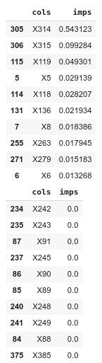

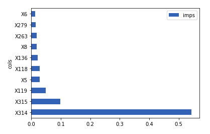
As we can see, X314 is by far the most important feature, X315 is a distant second, X119 is third, and the rest of the top 10 important features are really close. Please also note that there’s at least 10 features which are completely useless to our model and just occupy a lot of memory. We can now use this new knowledge to do feature selection.

我们可以看到，X314是迄今为止最重要的功能，X315是排在第二的，X119是第三，其余十大重要功能的确非常接近。另请注意，至少有10个功能对我们的模型完全没有用，只是占用了很多内存。现在，我们可以使用这一新知识来进行特征选择。

Since we have the importance of each feature (and not just their rankings), an easy way to identify these “useless” features would be to set a certain numerical threshold for the importance of our columns and only keep the ones above our threshold. A good value for this threshold can vary from dataset to dataset but in practice, 0.005 often works well (if you have time though, this is yet another hyperparameter waiting to be tuned):

由于我们具有每个功能的重要性(而不仅仅是它们的排名)，因此识别这些“无用”功能的简便方法是为列的重要性设置一个特定的数值阈值，而仅将其保持在阈值之上。此阈值的合适值可能因数据集而异，但实际上，0.005通常效果很好(如果有时间，这是另一个需要调整的超参数)：

to_keep = list(feat_imp[0.005<=feat_imp['imps']]['cols'])train_keep = train[to_keep+[dep_var]]

Let’s see how this affects our model’s score (in a perfect world, we would tune our hyperparameters each time we modify our dataset but in reality, that’d be inefficient and using the hyperparameters we found should work well):

让我们看一下这如何影响模型的得分(在理想情况下，每次修改数据集时我们都会调整超参数，但实际上这效率低下，使用我们发现的超参数应该可以正常工作)：

do_cross_val(RandomForestRegressor, train_keep,**rf_args)
Output:Cross validation scores: [0.563 0.576 0.566 0.586 0.578]
Cross validation average score: 0.574
Cross validation standard deviation: 0.008

We can see our overall score is about the same, but now we’re getting much more consistent scores during each iteration of cross-validation, which is important by itself. Just as important, though, is the fact that we now have 18 features instead of a whopping 376. Not only does this indicate faster training, but it also means we can now carefully examine each feature and do more rigorous exploratory data analysis, which will be the subject of a future article.

我们可以看到我们的总体分数大致相同，但是现在在每次交叉验证迭代期间我们都获得了更加一致的分数，这本身很重要。同样重要的是，我们现在拥有18个功能，而不是多达376个。这不仅表明培训速度更快，而且还意味着我们现在可以仔细检查每个功能并进行更严格的探索性数据分析，成为未来文章的主题。

Let’s make these changes to the original dataset:

让我们对原始数据集进行以下更改：

train = train[to_keep+[dep_var]]X = X[to_keep]

After this step, it’s almost guaranteed that the importance of each feature will change and so for the sake of understanding our data, we should calculate feature importances again (it should be noted the following is more trustworthy than the previous one):

完成此步骤后，几乎可以保证每个功能的重要性都会发生变化，因此为了理解我们的数据，我们应该再次计算功能的重要性(应该注意的是，以下内容比上一个更值得信赖)：

rf.fit(X, y)feat_imp = create_feat_imp(rf, X)plot_feat_imp(feat_imp)
Output: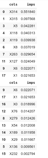

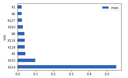
We can see in regards to X314 and X315, not much has changed but X119 is no longer the third most important feature and instead, it’s basically as important as the rest of the top 10 important features.

我们可以看到，对于X314和X315而言，变化不大，但是X119不再是第三重要的功能，它基本上与前十个重要功能中的其他功能一样重要。

We got rid of features that aren’t helpful when it comes to predicting the dependent variable. However, there’s one thing we didn’t consider: What if there are 2 separate columns that basically capture the same important thing? For instance, let’s say in this dataset, the factor that impacts the testing time of a vehicle is its speed, which is given to us in both kilometers and miles. Now, our model is going to place high values on both these columns and both their importances will be high, which means we wouldn’t have gotten rid of either using the above method. But there’s no point whatsoever in keeping both these features! So we obviously need a way to find out how correlated our features are, and that’s where Spearman’s rank-order correlation comes into play.

在预测因变量方面，我们摆脱了一些无用的功能。但是，我们没有考虑一件事：如果有2个单独的列基本上捕获了同一件重要的事情该怎么办？例如，在此数据集中，影响车辆测试时间的因素是其速度，它以公里和英里为单位给出。现在，我们的模型将在这两个列上都设置高值，并且它们的重要性都很高，这意味着使用以上方法我们都不会摆脱任何一个。但是，保留这两个功能毫无意义！因此，我们显然需要一种方法来找出我们的功能之间的相关性，而这正是Spearman的排名相关性发挥作用的地方。

斯皮尔曼等级相关 (Spearman’s Rank Correlation)

As I mentioned above, we need to see how correlated a group of features are (that is, how related are the values they capture). There are countless ways to do so, with my favorite being Spearman’s rank-order correlation (frankly, however, one would most likely get more or less the same result using any method.).

如前所述，我们需要查看一组功能之间的关联度(即它们捕获的值之间的关联度)。这样做的方法有无数种，其中我最喜欢的是Spearman的排名相关性(坦率地说，使用任何一种方法都可能或多或少地获得相同的结果。)

It is awfully easy to calculate and visualize our features’ correlations using SciPy and you can copy and paste the following lines of code with virtually no modifications for any dataset:

使用SciPy可以非常容易地计算和可视化我们的要素之间的相关性，并且您可以复制和粘贴以下代码行，而几乎无需修改任何数据集：

corr = np.round(scipy.stats.spearmanr(train).correlation, 4)corr_condensed = hc.distance.squareform(1-corr)z = hc.linkage(corr_condensed, method='average')fig = plt.figure(figsize=(16,10))dendrogram = hc.dendrogram(z, labels=train.columns, orientation='left', leaf_font_size=16)plt.show()
Output: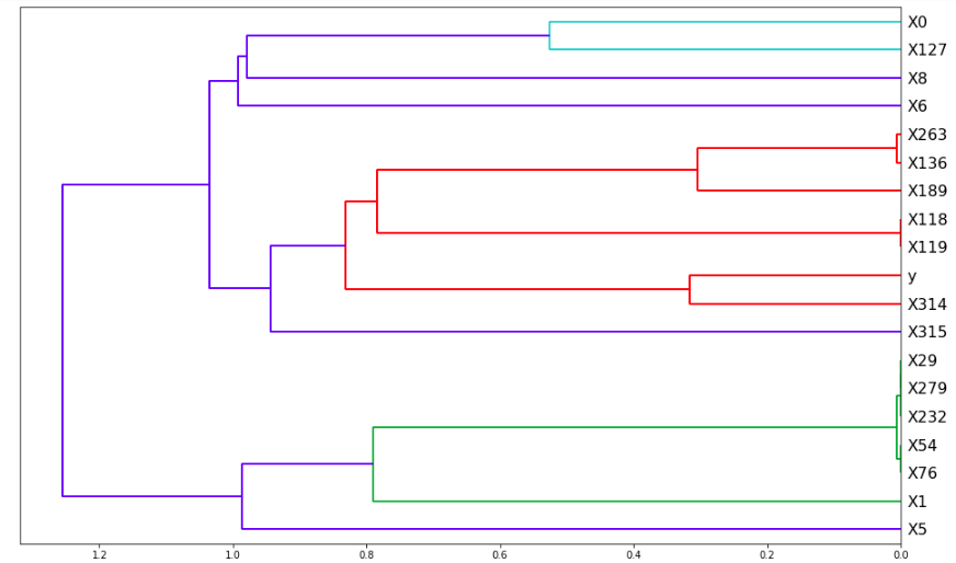

To interpret this, see where a group of features get merged (what value on the x-axis) and the lower that value is, the more correlated those two features are. For example, it looks like X0 and X127 merge at roughly x=0.55, whereas X118 and X119 merge at x=0. This means X118 and X119 are almost certainly capturing the same value but X0 and X127 are only somewhat related.

要对此进行解释，请查看在哪里合并了一组要素(x轴上的值)，并且该值越低，这两个要素的相关性就越高。例如，看起来X0和X127在大约x = 0.55处合并，而X118和X119在x = 0处合并。这意味着X118和X119几乎肯定会捕获相同的值，但是X0和X127只是有些相关。

Nonetheless, we can’t just drop X118 or X119 because sometimes, although the features are correlated, we need both of them and dropping either could cause a decrease in our model’s score. To overcome this issue, we can go through each feature in a group of features that are all correlated, do cross-validation but without that feature in our dataset, and see how that affects our score. From there, we can make informed decisions rather than just randomly dropping, say, X118 or X119:

尽管如此，我们不能只删除X118或X119，因为有时尽管功能是相关的，但我们都需要它们，而删除任何一个都可能导致模型得分降低。为了克服这个问题，我们可以遍历一组都相关的要素中的每个要素，进行交叉验证，但在我们的数据集中却没有该要素，然后看看它如何影响我们的得分。从那里，我们可以做出明智的决定，而不仅仅是随机丢弃，例如X118或X119：

# Groups of features which are highly correlatedto_remove = ['X232', 'X279', 'X29','X118', 'X119','X54', 'X76']for feat in to_remove:    print(feat)    do_cross_val(RandomForestRegressor, train.drop(feat, axis=1),**rf_args)
Output:X232 
Cross validation scores: [0.563 0.556 0.596 0.549 0.560]
Cross validation average score: 0.565
Cross validation standard deviation: 0.016
X279 
Cross validation scores: [0.605 0.592 0.512 0.551 0.596]
Cross validation average score: 0.571
Cross validation standard deviation: 0.034
X29
Cross validation scores: [0.611 0.478 0.600 0.569 0.600]
Cross validation average score: 0.572
Cross validation standard deviation: 0.048
X118
Cross validation scores: [0.514 0.470 0.637 0.599 0.600]
Cross validation average score: 0.564
Cross validation standard deviation: 0.061
X119
Cross validation scores: [0.446 0.623 0.574 0.456 0.598]
Cross validation average score: 0.539
Cross validation standard deviation: 0.073
X54
Cross validation scores: [0.563 0.510 0.487 0.446 0.627]
Cross validation average score: 0.527
Cross validation standard deviation: 0.063
X76 
Cross validation scores: [0.561 0.547 0.490  0.631 0.464]
Cross validation average score: 0.538
Cross validation standard deviation: 0.058

As shown, there’s not a single instance where our score or STD got better. We might be able to get away with removing X279 & X29 and the decline in our score would be about 0.003, which can be substituted by adding more decision trees. But please note that our STD could potentially get 6 times larger, which might prove to be troublesome later on. And anyhow, I’m pretty sure we can live with having 2 extra features so we’ll keep them.

如图所示，在任何情况下，我们的得分或性病都不会好转。我们也许可以摆脱X279和X29的困扰，而我们的得分下降大约为0.003，可以通过添加更多决策树来代替。但是请注意，我们的STD可能会增大6倍，这可能会在以后带来麻烦。而且，无论如何，我很确定我们可以使用2个额外的功能，因此我们将保留它们。

P.S: Although, in our case, there wasn’t a high amount of correlation between our features, that doesn’t imply that’s the case with every tabular dataset and you should definitely be on the watch for correlated features in your own projects.

PS：尽管在我们的案例中，我们的功能之间没有很高的关联性，但这并不意味着每个表格数据集都是如此，您一定要注意自己项目中的相关功能。

结论 (Conclusion)

In this part, we went through arguably the most important steps in this series: We chose the proper validation technique for our problem, we fine-tuned our Random Forest which, in turn, allowed us to do some heavy feature selection, reducing the number of columns by a magnitude of 20. In my modest opinion, you should for sure allocate a generous amount of your time for the things we did in this article and get comfortable with them.

在这一部分中，我们可以说是本系列中最重要的步骤：我们选择了适合我们问题的正确验证技术，并对我们的“随机森林”进行了微调，从而使我们能够进行一些繁重的特征选择，从而减少了数量列的数量最多为20。在我的谦虚意见中，您应该确保为本文中的工作分配大量的时间，并让他们感到满意。

In the next part (or possible next 2 parts), we’ll do exploratory feature analysis, which is an important part of every machine learning project. Although we might not end up increasing our score, we will be able to draw invaluable insights from our data, which is important by itself.

在下一部分(或可能的下两部分)中，我们将进行探索性特征分析，这是每个机器学习项目的重要组成部分。尽管我们可能最终不会提高得分，但我们将能够从我们的数据中获得宝贵的见解，这本身就很重要。

Please, if you have any questions or feedback at all, feel welcome to post them in the comments below and as always, thank you for reading!

请，如果您有任何疑问或反馈，欢迎在下面的评论中发表，并一如既往地感谢您的阅读！

Part 1: https://medium.com/python-in-plain-english/mercedes-benz-greener-manufacturing-part-1-basic-data-pre-processing-a32d17803064

第1部分： https ： //medium.com/python-in-plain-english/mercedes-benz-greener-manufacturing-part-1-basic-data-pre-processing-a32d17803064

Twitter: https://twitter.com/bobmcdear

推特： https : //twitter.com/bobmcdear

GitHub: https://github.com/bobmcdear

GitHub： https ： //github.com/bobmcdear