大数据工程师要学的编程_每个数据工程师都应了解的ml编程技巧，第2部分-CSDN博客

大数据工程师要学的编程

现实世界中的DS(DS IN THE REAL WORLD)

这篇文章是下面提到的继续。 (This post is in continuation with the one mentioned below.)

In the above post, I have presented some important programming takeaways to know and keep in mind while performing Machine Learning practices to make your implementation faster and effective. Following which we are going to see more of these hacks. Let us begin.

在上面的文章中，我介绍了一些重要的编程要点，它们在执行机器学习实践时要了解并牢记，以使您的实现更快，更有效。接下来，我们将看到更多这些技巧。让我们开始吧。

11.操纵宽和长数据帧： (11. Manipulating Wide & Long DataFrames:)

The most effective method for converting wide to long data and long to wide data is pandas.melt() and pandas.pivot_table() function respectively. You will not need anything else to manipulate long and wide data into one another other than these functions.

转换宽数据到长数据和长数据到宽数据的最有效方法分别是pandas.melt()和pandas.pivot_table()函数。除了这些功能之外，您不需要其他任何东西就可以将长而宽的数据相互转换。

一种。宽到长(融化) (a. Wide to Long (Melt))

>>> import pandas as pd
# create wide dataframe
>>> df_wide = pd.DataFrame(
...    {"student": ["Andy", "Bernie", "Cindy", "Deb"],
...     "school":  ["Z", "Y", "Z", "Y"],
...     "english": [66, 98, 61, 67],  # eng grades
...     "math":    [87, 48, 88, 47],  # math grades
...     "physics": [50, 30, 59, 54]   # physics grades
...    }
...  )
>>> df_wide
  student school  english  math  physics
0    Andy      Z       66    87       50
1  Bernie      Y       98    48       30
2   Cindy      Z       61    88       59
3     Deb      Y       67    47       54
>>> df_wide.melt(id_vars=["student", "school"],
...               var_name="subject",  # rename
...               value_name="score")  # rename
   student school  subject  score
0     Andy      Z  english     66
1   Bernie      Y  english     98
2    Cindy      Z  english     61
3      Deb      Y  english     67
4     Andy      Z     math     87
5   Bernie      Y     math     48
6    Cindy      Z     math     88
7      Deb      Y     math     47
8     Andy      Z  physics     50
9   Bernie      Y  physics     30
10   Cindy      Z  physics     59
11     Deb      Y  physics     54

b。长到宽(数据透视表) (b. Long to Wide (Pivot Table))

>>> import pandas as pd
# create long dataframe
>>> df_long = pd.DataFrame({
...         "student":
...             ["Andy", "Bernie", "Cindy", "Deb",
...              "Andy", "Bernie", "Cindy", "Deb",
...              "Andy", "Bernie", "Cindy", "Deb"],
...         "school":
...             ["Z", "Y", "Z", "Y",
...              "Z", "Y", "Z", "Y",
...              "Z", "Y", "Z", "Y"],
...         "class":
...             ["english", "english", "english", "english",
...              "math", "math", "math", "math",
...              "physics", "physics", "physics", "physics"],
...         "grade":
...             [66, 98, 61, 67,
...              87, 48, 88, 47,
...              50, 30, 59, 54]
... })
>>> df_long
   student school    class  grade
0     Andy      Z  english     66
1   Bernie      Y  english     98
2    Cindy      Z  english     61
3      Deb      Y  english     67
4     Andy      Z     math     87
5   Bernie      Y     math     48
6    Cindy      Z     math     88
7      Deb      Y     math     47
8     Andy      Z  physics     50
9   Bernie      Y  physics     30
10   Cindy      Z  physics     59
11     Deb      Y  physics     54
>>> df_long.pivot_table(index=["student", "school"], 
...                     columns='class', 
...                     values='grade')
class           english  math  physics
student school                        
Andy    Z            66    87       50
Bernie  Y            98    48       30
Cindy   Z            61    88       59
Deb     Y            67    47       54

12.交叉表： (12. Cross Tabulation:)

When you need to summarise the data, cross tabulation plays a great role to aggregate two or more factors and compute the frequency table for the values. It can be implemented with pandas.crosstab() function which also allows to find the normalized values while printing the output using ‘normalize’ parameter.

当您需要汇总数据时，交叉表在汇总两个或更多因素并计算这些值的频率表方面发挥着重要作用。可以使用pandas.crosstab()函数实现该函数，该函数还允许在使用'normalize'参数打印输出时查找归一化的值。

>>> import numpy as np
>>> import pandas as pd
>>> p = np.array(["s1", "s1", "s1", "s1", "b1", "b1",
...               "b1", "b1", "s1", "s1", "s1"], dtype=object)
>>> q = np.array(["one", "one", "one", "two", "one", "one",
...               "one", "two", "two", "two", "one"], dtype=object)
>>> r = np.array(["x", "x", "y", "x", "x", "y",
...               "y", "x", "y", "y", "y"], dtype=object)
>>> pd.crosstab(p, [q, r], rownames=['p'], colnames=['q', 'r'])
q  one    two   
r    x  y   x  y
p               
b1   1  2   1  0
s1   2  2   1  2# get normalized output values
>>> pd.crosstab(p, [q, r], rownames=['p'], colnames=['q', 'r'], normalize=True)
q        one                 two          
r          x         y         x         y
p                                         
b1  0.090909  0.181818  0.090909  0.000000
s1  0.181818  0.181818  0.090909  0.181818

13. Jupyter主题： (13. Jupyter Themes:)

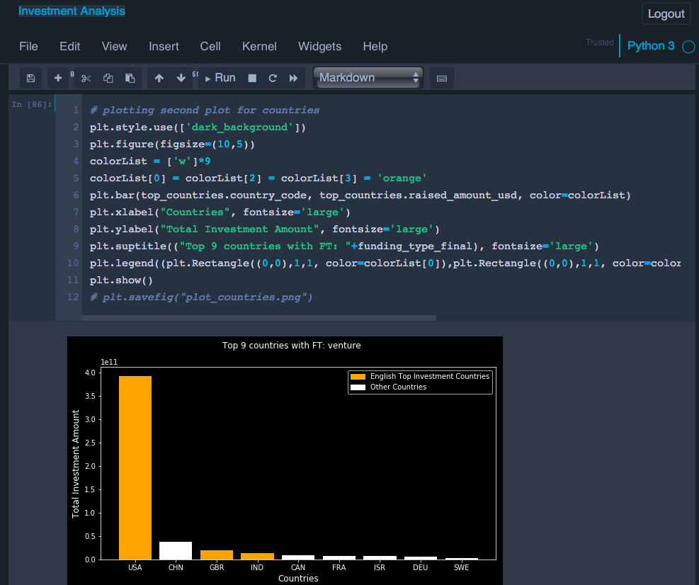
The one of the best libraries in Python is jupyterthemes that allows you to change and control the style of the notebook view that most of the ML practitioners work upon. As different themes like having dark mode, light mode, etc. or custom styling is preferred by most of the programmers and it can be achieved in Jupyter notebooks using jupyterthemes library.

Python中最好的库之一是jupyterthemes，它使您可以更改和控制大多数ML从业人员从事的笔记本视图的样式。由于大多数程序员都喜欢不同的主题，例如具有暗模式，亮模式等或自定义样式，因此可以使用jupyterthemes库在Jupyter笔记本中实现。

# pip install
$ pip install jupyterthemes# conda install
$ conda install -c conda-forge jupyterthemes# list available themes
$ jt -l
Available Themes:
   chesterish
   grade3
   gruvboxd
   gruvboxl
   monokai
   oceans16
   onedork
   solarizedd
   solarizedl# apply the theme
jt -t chesterish# reverse the theme
!jt -r

You can find more about it here on Github https://github.com/dunovank/jupyter-themes.

您可以在Github上找到更多有关它的信息https://github.com/dunovank/jupyter-themes 。

14.将分类转换为虚拟变量： (14. Convert Categorical to Dummy Variable:)

Using pandas.get_dummies() function, you can directly convert the categorical features in the DataFrame to Dummy variables along with drop_first=True to remove the first redundant column.

使用pandas.get_dummies()函数，可以将DataFrame中的分类功能与drop_first = True一起直接转换为Dummy变量，以删除第一个冗余列。

>>> import pandas as pd
>>> df = pd.DataFrame({'A': ['a', 'b', 'a'], 'B': ['b', 'a', 'c'],
...                     'C': [1, 2, 3]})>>> df
   A  B  C
0  a  b  1
1  b  a  2
2  a  c  3>>> pd.get_dummies(df[['A','B']])
   A_a  A_b  B_a  B_b  B_c
0    1    0    0    1    0
1    0    1    1    0    0
2    1    0    0    0    1>>> dummy = pd.get_dummies(df[['A','B']], drop_first=True)
>>> dummy
   A_b  B_b  B_c
0    0    1    0
1    1    0    0
2    0    0    1# concat dummy features to existing df
>>> df = pd.concat([df, dummy], axis=1)>>> df
   A  B  C  A_b  B_b  B_c
0  a  b  1    0    1    0
1  b  a  2    1    0    0
2  a  c  3    0    0    1

15.转换为数字： (15. Convert into Numeric:)

While loading dataset into pandas, sometimes the numeric column is taken object type and numeric operations cannot be performed on the same. In order to convert them to numeric, we can use pandas.to_numeric() function and update existing Series, or column in DataFrame.

在将数据集加载到熊猫中时，有时会将数字列作为对象类型，并且不能在同一列上执行数字操作。为了将它们转换为数字，我们可以使用pandas.to_numeric()函数并更新现有的Series或DataFrame中的列。

>>> import pandas as pd
>>> s = pd.Series(['1.0', '2', -3, '12', 5])
>>> s
0    1.0
1      2
2     -3
3     12
4      5
dtype: object>>> pd.to_numeric(s)
0     1.0
1     2.0
2    -3.0
3    12.0
4     5.0
dtype: float64>>> pd.to_numeric(s, downcast='signed')
0     1
1     2
2    -3
3    12
4     5
dtype: int8

16.分层采样/拆分： (16. Stratified Sampling/Splitting:)

When splitting the dataset, we need to obtain sample population in data splits at times. It is more effective when the classes are not balanced enough in the dataset. In sklearn.model_selection.train_test_split() function, a parameter named “stratify” can be set with target class feature to correctly split the data with same ratio as present in unsplitted dataset for different classes.

拆分数据集时，我们有时需要获取数据拆分中的样本总体。当类在数据集中不够平衡时，它会更有效。在sklearn.model_selection .train_test_split()函数中，可以使用目标类别功能设置名为“ stratify ”的参数，以与未分割数据集中不同类别的比率正确分割数据。

from sklearn.model_selection import train_test_split
X_train, X_test, y_train, y_test = train_test_split(X, y,
                                                    stratify=y, 
                                                    test_size=0.25)

17.按类型选择特征： (17. Selecting Features By Type:)

In most of the datasets, we have both types of columns, i.e. Numerical, and Non-Numerical. We often have the need to extract only the numerical columns or categorical columns in the dataset and perform some visualization functions or custom manipulations on the same. In pandas library, we have DataFrame.select_dtypes() function which selects the specific columns from the given dataset that matches the specified datatype.

在大多数数据集中，我们有两种类型的列，即数值列和非数值列。我们经常需要仅提取数据集中的数字列或分类列，并对它们执行一些可视化功能或自定义操作。在熊猫库中，我们具有DataFrame.select_dtypes()函数，该函数从给定的数据集中选择与指定数据类型匹配的特定列。

>>> import pandas as pd
>>> df = pd.DataFrame({'a': [1, 2] * 3,
...                     'b': [True, False] * 3,
...                     'c': [1.0, 2.0] * 3})
>>> df
   a      b    c
0  1   True  1.0
1  2  False  2.0
2  1   True  1.0
3  2  False  2.0
4  1   True  1.0
5  2  False  2.0>>> df.select_dtypes(include='bool')
       b
0   True
1  False
2   True
3  False
4   True
5  False>>> df.select_dtypes(include=['float64'])
     c
0  1.0
1  2.0
2  1.0
3  2.0
4  1.0
5  2.0>>> df.select_dtypes(exclude=['int64'])
       b    c
0   True  1.0
1  False  2.0
2   True  1.0
3  False  2.0
4   True  1.0
5  False  2.0

18. RandomizedSearchCV： (18. RandomizedSearchCV:)

RandomizedSearchCV is a function from sklearn.model_selectionclass that is used to determine random set of hyperparameters for the mentioned learning algorithm, it randomly selects different values for each hyperparameter provided to tune and applied cross-validations on each selected value and determine the best one of them using different scoring mechanism provided while searching.

RandomizedSearchCV是sklearn.model_selection类的一个函数，用于为所提到的学习算法确定随机的超参数集，它为提供的每个超参数随机选择不同的值，以调整和应用对每个选定值的交叉验证，并确定最佳选择之一。他们使用搜索时提供的不同评分机制。

>>> from sklearn.datasets import load_iris
>>> from sklearn.linear_model import LogisticRegression
>>> from sklearn.model_selection import RandomizedSearchCV
>>> from scipy.stats import uniform
>>> iris = load_iris()
>>> logistic = LogisticRegression(solver='saga', tol=1e-2, 
...                               max_iter=300,random_state=12)
>>> distributions = dict(C=uniform(loc=0, scale=4),
...                      penalty=['l2', 'l1'])>>> clf = RandomizedSearchCV(logistic, distributions, random_state=0)>>> search = clf.fit(iris.data, iris.target)>>> search.best_params_
{'C': 2..., 'penalty': 'l1'}

19.魔术功能-历史记录： (19. Magic function — %history:)

A batch of previously ran commands in the notebook can be accessed using ‘%history’ magic function. This will provide all previously executed commands and can be provided custom options to select the specific history commands which you can check using ‘%history?’ in jupyter notebook.

可以使用'％history'魔术功能访问笔记本中一批以前运行的命令。这将提供所有以前执行的命令，并可以提供自定义选项以选择特定的历史命令，您可以使用'％history？'进行检查。在jupyter笔记本中。

In [1]: import math

In [2]: math.sin(2)
Out[2]: 0.9092974268256817

In [3]: math.cos(2)
Out[3]: -0.4161468365471424In [16]: %history -n 1-3
   1: import math
   2: math.sin(2)
   3: math.cos(2)

20.下划线快捷方式(_)： (20. Underscore Shortcuts (_):)

In python, you can directly print the last output sent by the interpreter using print(_) function with underscore. This might not be that helpful, but in IPython (jupyter notebook), this feature has been extended and you can print any nth last output using n underscores within print() function. E.g. print(__) with two underscores will give you second-to-last output which skips all command that has no output.

在python中，您可以使用带下划线的print(_)函数直接打印解释器发送的最后输出。这可能没有帮助，但是在IPython(jupyter笔记本)中，此功能已得到扩展，您可以在print()函数中使用n下划线打印任何n个最后输出。例如带有两个下划线的print(__)将为您提供倒数第二个输出，该输出将跳过所有没有输出的命令。

Also, another is underscore followed by line number prints the associated output.

此外，另一个是下划线，其后是行号，以打印相关的输出。

In [1]: import math

In [2]: math.sin(2)
Out[2]: 0.9092974268256817

In [3]: math.cos(2)
Out[3]: -0.4161468365471424In [4]: print(_)
-0.4161468365471424

In [5]: print(__)
0.9092974268256817In [6]: _2
Out[13]: 0.9092974268256817

That’s all for now. I will present more of these important hacks/functions that every data engineer should know about in more next few parts.

目前为止就这样了。我将在接下来的几个部分中介绍每个数据工程师都应该了解的这些重要的技巧/功能。

Stay tuned.

敬请关注。

Thanks for reading. You can find my other Machine Learning related posts here.

谢谢阅读。您可以在这里找到我其他与机器学习有关的帖子。

I hope this post has been useful. I appreciate feedback and constructive criticism. If you want to talk about this article or other related topics, you can drop me a text here or at LinkedIn.

希望这篇文章对您有所帮助。我感谢反馈和建设性的批评。如果您想谈论本文或其他相关主题，可以在此处或在LinkedIn上给我发短信。