


机器学习 物理引擎
我们如何预测冠状物质抛射? (How Can We Predict Coronal Mass Ejections?)
Coronal Mass Ejection (CME) is a significant release of plasma and magnetic field from the Sun into interplanetary space. CMEs are the primary source of strong geomagnetic storms, which are major disturbances of Earth’s magnetosphere that can lead to massive damage of satellites, power grids, and telecommunications/navigation systems. Therefore, it is important to forecast geomagnetic storms — and CMEs that lead to such events — in a reliable way. In this article, I share my way of applying machine learning techniques to predicting CMEs.
日冕物质抛射 (CME)是从太阳到行星际空间的大量等离子体和磁场释放。 CME是强地磁风暴的主要来源,强地磁风暴是地球磁层的主要扰动,可能导致卫星,电网和电信/导航系统的大量破坏。 因此,以可靠的方式预测地磁风暴以及导致此类事件的CME非常重要。 在本文中,我分享了将机器学习技术应用于CME预测的方法。
This article provides a step-by-step overview of how to access solar data, preprocess it, and build a Topological Data Analysis-based classifier. We then discuss the performance of the classifier at the end.
本文分步概述了如何访问太阳能数据,对其进行预处理以及构建基于拓扑数据分析的分类器。 然后,我们最后讨论分类器的性能。

介绍 (Introduction)
A Coronal Mass Ejection (CME) is a significant release of plasma and magnetic field from the Sun into interplanetary space. Despite the progress in numerical modeling, it is still unclear which conditions will produce a CME; however, it is known that CMEs and solar flares are associated as “a single magnetically driven event” (Webb & Howard 2012).
日冕物质抛射(CME)是从太阳到行星际空间的大量等离子体和磁场释放。 尽管数值建模取得了进展,但尚不清楚哪些条件将产生CME。 然而,众所周知,CME和太阳耀斑被称为“单个磁驱动事件”( Webb&Howard 2012 )。
In general, the more energetic a flare, the more likely it is to be associated with a CME (Yashiro et al. 2005) — but this is not a rule. For example, Sun et al. (2015) found that the largest active region in the last 24 years produced 6 X-class flares but not a single observed CME.
通常,耀斑越活跃,就越有可能与CME相关联( Yashiro et al。2005 )-但这不是规则。 例如, Sun等。 (2015年 )发现,过去24年中最大的活跃区域产生了6个X级耀斑,但没有观测到一个CME。
Here, we use a topological data analysis-based classifier to predict whether an M- or X-class flaring active region will produce a CME.
在这里,我们使用基于拓扑数据分析的分类器来预测M级或X级扩口活动区域是否会产生CME。
To do this analysis, we’ll look at every active region observed by the Helioseismic and Magnetic Imager instrument on NASA’s Solar Dynamics Observatory (SDO) satellite over the last nine years. Each active region is characterized by a set of features that parameterize its magnetic field. One feature, for example, is the total energy contained within an active region. Another is the total flux through an active region. We use 18 features, which are calculated every 12 minutes throughout an active region’s lifetime. See Bobra et al., 2014 for more information about the calculation of these features.
为了进行此分析,我们将查看过去9年中在美国国家航空航天局(NASA)的太阳动力学天文台(SDO)卫星上用Heismesism and Magnetic Imager仪器观测到的每个活动区域。 每个有源区域的特征是一组参数化其磁场的特征。 例如,一个特征是有效区域内包含的总能量。 另一个是通过有源区域的总通量。 我们使用18个功能,这些功能在活动区域的整个生命周期中每12分钟计算一次。 有关这些功能的计算的更多信息,请参见Bobra等人,2014年 。
We’ll then ascribe each active region to one of two classes:
然后,我们将每个活动区域归为以下两个类别之一:
1. The positive class contains flaring active regions that did produce a CME.
1.阳性类别包含确实产生CME的喇叭形活性区域。
2. The negative class contains flaring active regions that did not produce a CME.
2.阴性类别包含未产生CME的张开的活性区域。
数据 (Data)
导入库 (Importing libraries)
Let’s implement in Python what we just described above. First, we’ll import some modules.
让我们用Python实现上面刚刚描述的内容。 首先,我们将导入一些模块。
import numpy as np
import matplotlib.pylab as plt
import matplotlib.mlab as mlab
import pandas as pd
import mpld3
import requests
import urllib
import json
from datetime import datetime as dt_obj
from datetime import timedelta
from mpld3 import plugins
from sunpy.time import TimeRange
import sunpy.instr.goes
from sklearn.model_selection import train_test_split
from sklearn.preprocessing import OneHotEncoder
import tensorflow as tf


pd.set_option('display.max_rows', 500)
%matplotlib inline
%config InlineBackend.figure_format = 'retina'
Now we’ll collect the data. The data come from the following sources:
现在,我们将收集数据。 数据来自以下来源:
- CME data from SOHO/LASCO and STEREO/SECCHI coronographs,which can be accesed from the DONKI database at NASA Goddard. This tells us if an active region has produced a CME or not. 来自SOHO / LASCO和STEREO / SECCHI冠冕仪的CME数据可从NASA Goddard的DONKI数据库获取。 这告诉我们活动区域是否生成了CME。
- Flare data from the GOES flare catalog at NOAA, which can be accessed with the sunpy.instr.goes.get_event_list() function. This tells us if an active region produced a flare or not. 来自NOAA的GOES火炬目录中的火炬数据,可以使用sunpy.instr.goes.get_event_list()函数进行访问。 这告诉我们活动区域是否产生了耀斑。
- Active region data from the Solar Dynamics Observatory’s Heliosesmic and Magnetic Im- ager instrument, which can be accessed from the JSOC database via a JSON API. This gives us the features characterizing each active region. 来自太阳动力天文台的日地电磁成像仪的活动区域数据,可以通过JSON API从JSOC数据库访问。 这为我们提供了表征每个活动区域的功能。
步骤1:为肯定类别收集数据 (Step 1: Collecting Data for the Positive Class)
We first query the DONKI database to get the data associated with the positive class.
我们首先查询DONKI数据库以获取与肯定类关联的数据。
# request the data
baseurl = "https://kauai.ccmc.gsfc.nasa.gov/DONKI/WS/get/FLR?" t_start = "2010-05-01"
t_end = "2019-07-01"
url = baseurl+"startDate="+t_start+"&endDate="+t_end
# if there's no response at this time, print warning
response = requests.get(url)
if response.status_code != 200:
    print('cannot successfully get an http response')

# read the data
print("Getting data from", url) df = pd.read_json(url)
# select flares associated with a linked event (SEP or CME), and # select only M or X-class flares
events_list = df.loc[df['classType'].str.contains(
"M|X") & ~df['linkedEvents'].isnull()]
# drop all rows that don't satisfy the above conditions
events_list = events_list.reset_index(drop=True)


# drop the rows that aren't linked to CME events
for i in range(events_list.shape[0]):
value = events_list.loc[i]['linkedEvents'][0]['activityID'] if not "CME" in value:
        print(value, "not a CME, dropping row")
events_list = events_list.drop([i]) events_list = events_list.reset_index(drop=True)
We then convert the peakTime column in the events_list dataframe from a string into a datetime object:
然后,我们将events_list数据帧中的peakTime列从字符串转换为datetime对象:
def parse_tai_string(tstr):
    year = int(tstr[:4])
    month = int(tstr[5:7])
    day = int(tstr[8:10])
    hour = int(tstr[11:13])
    minute = int(tstr[14:16])
    return dt_obj(year, month, day, hour, minute)


for i in range(events_list.shape[0]):
    events_list['peakTime'].iloc[i] = parse_tai_string(
        events_list['peakTime'].iloc[i])
Case 1: the CME and flare exist but NOAA active region number does not exist in the DONKI database.
情况1:存在CME和耀斑,但DONKI数据库中不存在NOAA活动区域编号。
# Case 1: check if there was a flare associated with an Active Region (AR) in GOES database but the AR ID wasn't included in the DONKI database


#If there was a flare not associated with an AR, we drop that row because we can't analyze it


number_of_donki_mistakes = 0  # count the number of DONKI mistakes
# create an empty array to hold row numbers to drop at the end
event_list_drops = []


for i in range(events_list.shape[0]):
    if (np.isnan(events_list.loc[i]['activeRegionNum'])):
        time = events_list['peakTime'].iloc[i]
        time_range = TimeRange(time, time)
        listofresults = sunpy.instr.goes.get_goes_event_list(time_range, 'M1') #'M1' is a GOES class filter specifying a minimum GOES class for inclusion in the list, e.g. ‘M1’, ‘X2’.
        if (listofresults[0]['noaa_active_region'] == 0):
            print(events_list.loc[i]['activeRegionNum'], events_list.loc[i]
                  ['classType'], "has no match in the GOES flare database ; dropping row.")
            event_list_drops.append(i)
            number_of_donki_mistakes += 1
            continue
        else:
            print("Missing NOAA number:", events_list['activeRegionNum'].iloc[i], events_list['classType'].iloc[i],
                  events_list['peakTime'].iloc[i], "should be", listofresults[0]['noaa_active_region'], "; changing now.")
            events_list['activeRegionNum'].iloc[i] = listofresults[0]['noaa_active_region']
            number_of_donki_mistakes += 1


# Drop the rows for which there is no active region number in both the DONKI and GOES flare databases
events_list = events_list.drop(event_list_drops)
events_list = events_list.reset_index(drop=True)
print('There are', number_of_donki_mistakes, 'DONKI mistakes so far.')
Now we take all the data from the GOES database in preparation for checking Cases 2 and 3.
现在,我们从GOES数据库中获取所有数据,以准备检查案例2和3。
# Take all the data from the GOES database
time_range = TimeRange(t_start, t_end)
listofresults = sunpy.instr.goes.get_goes_event_list(time_range, 'M1')
print('Grabbed all the GOES data; there are', len(listofresults), 'events.')
Case 2: the NOAA active region number is wrong in the DONKI database.
情况2: DONKI数据库中的NOAA活动区域编号错误。
# Case 2: NOAA active region number is wrong in DONKI database


# collect all the peak flares times in the NOAA database
peak_times_noaa = [item["peak_time"] for item in listofresults]


for i in range(events_list.shape[0]):
    # check if a particular DONKI flare peak time is also in the NOAA database
    peak_time_donki = events_list['peakTime'].iloc[i]
    if peak_time_donki in peak_times_noaa:
        index = peak_times_noaa.index(peak_time_donki)
    else:
        continue
    # ignore NOAA active region numbers equal to zero
    if (listofresults[index]['noaa_active_region'] == 0):
        continue
    # if yes, check if the DONKI and NOAA active region numbers match up for this peak time
    # if they don't, flag this peak time and replace the DONKI number with the NOAA number
    if (listofresults[index]['noaa_active_region'] != events_list['activeRegionNum'].iloc[i].astype(int)):
        print('Messed up NOAA number:', events_list['activeRegionNum'].iloc[i].astype(int), events_list['classType'].iloc[i],
              events_list['peakTime'].iloc[i], "should be", listofresults[index]['noaa_active_region'], "; changing now.")
        events_list['activeRegionNum'].iloc[i] = listofresults[index]['noaa_active_region']
        number_of_donki_mistakes += 1
print('There are', number_of_donki_mistakes, 'DONKI mistakes so far.')
Case 3: the flare peak time is wrong in the DONKI database.
情况3:在DONKI数据库中,火炬高峰时间错误。
# Case 3: The flare peak time is wrong in the DONKI database.


# create an empty array to hold row numbers to drop at the end
event_list_drops = []


active_region_numbers_noaa = [item["noaa_active_region"]
                              for item in listofresults]
flare_classes_noaa = [item["goes_class"] for item in listofresults]


for i in range(events_list.shape[0]):
    # check if a particular DONKI flare peak time is also in the NOAA database
    peak_time_donki = events_list['peakTime'].iloc[i]
    if not peak_time_donki in peak_times_noaa:
        active_region_number_donki = int(
            events_list['activeRegionNum'].iloc[i])

        flare_class_donki = events_list['classType'].iloc[i]

        flare_class_indices = [i for i, x in enumerate(
            flare_classes_noaa) if x == flare_class_donki]

        active_region_indices = [i for i, x in enumerate(
            active_region_numbers_noaa) if x == active_region_number_donki]


        common_indices = list(
            set(flare_class_indices).intersection(active_region_indices))
        if common_indices:
            print("Messed up time:", int(events_list['activeRegionNum'].iloc[i]), events_list['classType'].iloc[i],
                  events_list['peakTime'].iloc[i], "should be", peak_times_noaa[common_indices[0]], "; changing now.")
            events_list['peakTime'].iloc[i] = peak_times_noaa[common_indices[0]]
            number_of_donki_mistakes += 1
        if not common_indices:
            print("DONKI flare peak time",
                  events_list['peakTime'].iloc[i], "has no match; dropping row.")
            event_list_drops.append(i)
            number_of_donki_mistakes += 1


# Drop the rows for which the NOAA active region number and flare class associated with
# the messed-up flare peak time in the DONKI database has no match in the GOES flare database
events_list = events_list.drop(event_list_drops)
events_list = events_list.reset_index(drop=True)


# Create a list of corrected flare peak times
peak_times_donki = [events_list['peakTime'].iloc[i]
                    for i in range(events_list.shape[0])]


print('There are', number_of_donki_mistakes, 'DONKI mistakes so far.')
Now let’s query the JSOC database to see if there are active region parameters at the time of the flare. First we read the following file to map NOAA active region numbers to HARPNUMs (a HARP, or an HMI Active Region Patch, is the preferred numbering system for the HMI active regions as they appear in the magnetic field data before NOAA observes them in white light):
现在,让我们查询JSOC数据库,以查看在爆发时是否存在活动区域参数。 首先,我们阅读以下文件以将NOAA有源区域编号映射到HARPNUM(HARP有源区域补丁程序是HARP或HMI有源区域补丁,这是HMI有源区域出现在磁场数据中的首选编号系统,因为NOAA在白光下观察到它们之前) ):
answer = pd.read_csv(
    'http://jsoc.stanford.edu/doc/data/hmi/harpnum_to_noaa/all_harps_with_noaa_ars.txt', sep=' ')


#one HARP number can have more than one NOAA AR numbers
We now determine at which times before a CME happens we’d like to collect AR region data. For this, we set a variable called timedelayvariable[i] where i indicate at what time we collect AR region data (i.e. 6, 12, 18, 24 hr before a CME happens) :
现在,我们确定要在CME发生之前的哪些时间收集AR区域数据。 为此,我们设置了一个名为timedelayvariable[i]的变量,其中我指示何时采集AR区域数据(即CME发生前的6、12、18、24小时):
timedelayvariable6 = 6
timedelayvariable12 = 12
timedelayvariable18 = 18
timedelayvariable24 = 24
Now, we’ll subtract timedelayvariable from the GOES Peak Time and re-format the datetime object into a string that JSOC can understand:
现在,我们将从GOES峰值时间中减去timedelayvariable并将日期时间对象重新格式化为JSOC可以理解的字符串:
t_rec24 = [(events_list['peakTime'].iloc[i] - timedelta(hours=timedelayvariable24)
          ).strftime('%Y.%m.%d_%H:%M_TAI') for i in range(events_list.shape[0])]
t_rec18 = [(events_list['peakTime'].iloc[i] - timedelta(hours=timedelayvariable18)
          ).strftime('%Y.%m.%d_%H:%M_TAI') for i in range(events_list.shape[0])]
t_rec12 = [(events_list['peakTime'].iloc[i] - timedelta(hours=timedelayvariable12)
          ).strftime('%Y.%m.%d_%H:%M_TAI') for i in range(events_list.shape[0])]
t_rec6 = [(events_list['peakTime'].iloc[i] - timedelta(hours=timedelayvariable6)
          ).strftime('%Y.%m.%d_%H:%M_TAI') for i in range(events_list.shape[0])]
Next, we can take the SDO data from the JSOC database by executing the JSON queries. We are selecting data that satisfies the following criteria: The data has to be 1) disambiguated with a version of the disambiguation module greater than 1.1, 2) taken while the orbital velocity of the spacecraft is less than 3500 m/s, 3) of a high quality, and 4) within 70 degrees of central meridian. If the data pass all these tests, they are stuffed into one of two lists: one for the positive class (CME_data) and one for the negative class (no_CME_data).
接下来,我们可以通过执行JSON查询从JSOC数据库中获取SDO数据。 我们正在选择满足以下条件的数据:数据必须是:1)使用大于1.1的消歧模块版本进行了消歧,2)在航天器的轨道速度小于3500 m / s时获取,3) 4)中心子午线70度以内。 如果数据通过所有这些测试,则将它们填充到两个列表之一中:一个用于肯定类(CME_data),另一个用于否定类(no_CME_data)。
def get_the_jsoc_data_for_rnn(event_count, t_rec6, t_rec12, t_rec18, t_rec24):


    """
    Parameters
    ----------
    event_count: number of events
                 int

    t_rec[i], where i is in [6,12,18,24]:       list of times, one associated with each event in event_count
                 list of strings in JSOC format ('%Y.%m.%d_%H:%M_TAI')

    """


    catalog_data = []

    classification = []


    for i in range(event_count):


        print("=====", i, "=====")
        # next match NOAA_ARS to HARPNUM
        idx = answer[answer['NOAA_ARS'].str.contains(
            str(int(listofactiveregions[i])))]


        # if there's no HARPNUM, quit
        if (idx.empty == True):
            print('skip: there are no matching HARPNUMs for',
                  str(int(listofactiveregions[i])))
            continue


        # construct jsoc_info queries and query jsoc database; we are querying for 25 keywords


        url6 = "http://jsoc.stanford.edu/cgi-bin/ajax/jsoc_info?ds=hmi.sharp_720s["+str(
            idx.HARPNUM.values[0])+"]["+t_rec6[i]+"][? (CODEVER7 !~ '1.1 ') and (abs(OBS_VR)< 3500) and (QUALITY<65536) ?]&op=rs_list&key=USFLUX,MEANGBT,MEANJZH,MEANPOT,SHRGT45,TOTUSJH,MEANGBH,MEANALP,MEANGAM,MEANGBZ,MEANJZD,TOTUSJZ,SAVNCPP,TOTPOT,MEANSHR,AREA_ACR,R_VALUE,ABSNJZH"
        response6 = requests.get(url6)


        url12 = "http://jsoc.stanford.edu/cgi-bin/ajax/jsoc_info?ds=hmi.sharp_720s["+str(
            idx.HARPNUM.values[0])+"]["+t_rec12[i]+"][? (CODEVER7 !~ '1.1 ') and (abs(OBS_VR)< 3500) and (QUALITY<65536) ?]&op=rs_list&key=USFLUX,MEANGBT,MEANJZH,MEANPOT,SHRGT45,TOTUSJH,MEANGBH,MEANALP,MEANGAM,MEANGBZ,MEANJZD,TOTUSJZ,SAVNCPP,TOTPOT,MEANSHR,AREA_ACR,R_VALUE,ABSNJZH"
        response12 = requests.get(url12)


        url18 = "http://jsoc.stanford.edu/cgi-bin/ajax/jsoc_info?ds=hmi.sharp_720s["+str(
            idx.HARPNUM.values[0])+"]["+t_rec18[i]+"][? (CODEVER7 !~ '1.1 ') and (abs(OBS_VR)< 3500) and (QUALITY<65536) ?]&op=rs_list&key=USFLUX,MEANGBT,MEANJZH,MEANPOT,SHRGT45,TOTUSJH,MEANGBH,MEANALP,MEANGAM,MEANGBZ,MEANJZD,TOTUSJZ,SAVNCPP,TOTPOT,MEANSHR,AREA_ACR,R_VALUE,ABSNJZH"
        response18 = requests.get(url18)


        url24 = "http://jsoc.stanford.edu/cgi-bin/ajax/jsoc_info?ds=hmi.sharp_720s["+str(
            idx.HARPNUM.values[0])+"]["+t_rec24[i]+"][? (CODEVER7 !~ '1.1 ') and (abs(OBS_VR)< 3500) and (QUALITY<65536) ?]&op=rs_list&key=USFLUX,MEANGBT,MEANJZH,MEANPOT,SHRGT45,TOTUSJH,MEANGBH,MEANALP,MEANGAM,MEANGBZ,MEANJZD,TOTUSJZ,SAVNCPP,TOTPOT,MEANSHR,AREA_ACR,R_VALUE,ABSNJZH"
        response24 = requests.get(url24)


        # if there's no response at this time, quit


        if (response6.status_code != 200) or (response12.status_code != 200) or (response18.status_code != 200) or (response24.status_code != 200):
            print('skip: cannot successfully get an http response')
            continue


        # read the JSON output


        data6 = response6.json()
        data12 = response12.json()
        data18 = response18.json()
        data24 = response24.json()

        if (data6['count'] == 0) or (data12['count'] == 0) or (data18['count'] == 0) or (data24['count'] == 0):
            print('skip: there are no data for HARPNUM',
                  idx.HARPNUM.values[0], 'at time 24h', t_rec24[i])
            continue


        # check to see if the active region is too close to the limb
        # we can compute the latitude of an active region in stonyhurst coordinates as follows:
        # latitude_stonyhurst = CRVAL1 - CRLN_OBS
        # for this we have to query the CEA series (but above we queried the other series as the CEA series does not have CODEVER5 in it)


        url6 = "http://jsoc.stanford.edu/cgi-bin/ajax/jsoc_info?ds=hmi.sharp_cea_720s["+str(
            idx.HARPNUM.values[0])+"]["+t_rec6[i]+"][? (abs(OBS_VR)< 3500) and (QUALITY<65536) ?]&op=rs_list&key=CRVAL1,CRLN_OBS"
        response6 = requests.get(url6)


        url12 = "http://jsoc.stanford.edu/cgi-bin/ajax/jsoc_info?ds=hmi.sharp_cea_720s["+str(
            idx.HARPNUM.values[0])+"]["+t_rec12[i]+"][? (abs(OBS_VR)< 3500) and (QUALITY<65536) ?]&op=rs_list&key=CRVAL1,CRLN_OBS"
        response12 = requests.get(url12)


        url18 = "http://jsoc.stanford.edu/cgi-bin/ajax/jsoc_info?ds=hmi.sharp_cea_720s["+str(
            idx.HARPNUM.values[0])+"]["+t_rec18[i]+"][? (abs(OBS_VR)< 3500) and (QUALITY<65536) ?]&op=rs_list&key=CRVAL1,CRLN_OBS"
        response18 = requests.get(url18)


        url24 = "http://jsoc.stanford.edu/cgi-bin/ajax/jsoc_info?ds=hmi.sharp_cea_720s["+str(
            idx.HARPNUM.values[0])+"]["+t_rec24[i]+"][? (abs(OBS_VR)< 3500) and (QUALITY<65536) ?]&op=rs_list&key=CRVAL1,CRLN_OBS"
        response24 = requests.get(url24)

        if (response6.status_code != 200) or (response12.status_code != 200) or (response18.status_code != 200) or (response24.status_code != 200):
            print('skip: failed to find CEA JSOC data for HARPNUM',
                  idx.HARPNUM.values[0], 'at time 24 hr before an event', t_rec24[i])
            continue


        # read the JSON output


        latitude_information6 = response6.json()
        latitude_information12 = response12.json()
        latitude_information18 = response18.json()
        latitude_information24 = response24.json()

        if (latitude_information6['count'] == 0) or (latitude_information12['count'] == 0) or (latitude_information18['count'] == 0) or (latitude_information24['count'] == 0):
            print('skip: there are no data for HARPNUM',
                  idx.HARPNUM.values[0], 'at time 24 hr before an event', t_rec24[i])
            continue


        CRVAL1_6 = float(latitude_information6['keywords'][0]['values'][0])
        CRLN_OBS_6 = float(latitude_information6['keywords'][1]['values'][0])
        CRVAL1_12 = float(latitude_information12['keywords'][0]['values'][0])
        CRLN_OBS_12 = float(latitude_information12['keywords'][1]['values'][0])
        CRVAL1_18 = float(latitude_information18['keywords'][0]['values'][0])
        CRLN_OBS_18 = float(latitude_information18['keywords'][1]['values'][0])
        CRVAL1_24 = float(latitude_information24['keywords'][0]['values'][0])
        CRLN_OBS_24 = float(latitude_information24['keywords'][1]['values'][0])

        if (np.absolute(CRVAL1_6 - CRLN_OBS_6) > 70.0) or (np.absolute(CRVAL1_12 - CRLN_OBS_12) > 70.0) or (np.absolute(CRVAL1_18 - CRLN_OBS_18) > 70.0) or (np.absolute(CRVAL1_24 - CRLN_OBS_24) > 70.0):
            print('skip: latitude is out of range for HARPNUM',
                  idx.HARPNUM.values[0], 'at time 24 hr before an event', t_rec24[i])
            continue

        if  ('MISSING' in str(data6['keywords'])) or ('MISSING' in str(data12['keywords'])) or ('MISSING' in str(data18['keywords'])) or ('MISSING' in str(data24['keywords'])):
            print('skip: there are some missing keywords for HARPNUM',
                 idx.HARPNUM.values[0], 'at time 24 hr before an event', t_rec24[i])
            continue


        print('accept NOAA Active Region number', str(int(
            listofactiveregions[i])), 'and HARPNUM', idx.HARPNUM.values[0], 'at time 24 hr before an event', t_rec24[i])


        individual_flare_data6 = []
        for j in range(18):
            individual_flare_data6.append(
                float(data6['keywords'][j]['values'][0]))
        individual_flare_data12 = []
        for j in range(18):
            individual_flare_data12.append(
                float(data12['keywords'][j]['values'][0]))
        individual_flare_data18 = []
        for j in range(18):
            individual_flare_data18.append(
                float(data18['keywords'][j]['values'][0]))
        individual_flare_data24 = []
        for j in range(18):
            individual_flare_data24.append(
                float(data24['keywords'][j]['values'][0]))

        cat_data = []
        cat_data.extend([np.array(individual_flare_data6), np.array(individual_flare_data12), np.array(individual_flare_data18), np.array(individual_flare_data24)])


        print ('=================================')
        catalog_data.append(np.array(cat_data))
        print (np.array(catalog_data).shape)

        single_class_instance = [idx.HARPNUM.values[0], str(
            int(listofactiveregions[i])), listofgoesclasses[i], t_rec6[i], t_rec12[i], t_rec18[i], t_rec24[i]]
        classification.append(single_class_instance)

    return np.array(catalog_data), classification
Now we prepare data to be fed into the function and call the function:
现在,我们准备要输入到函数中的数据并调用该函数:
listofactiveregions = list(events_list['activeRegionNum'].values.flatten())
listofgoesclasses = list(events_list['classType'].values.flatten())


positive_result = get_the_jsoc_data_for_rnn(events_list.shape[0], t_rec6, t_rec12, t_rec18, t_rec24)
步骤2:收集负面类的数据 (Step 2: Collecting Data for the Negative Class)
To gather the examples for the negative class, we only need to:
要收集否定类的示例,我们只需要:
- Query the GOES database for all solar flares during our time of interest, and 在我们感兴趣的时间查询GOES数据库中的所有太阳耀斑,以及
- Select the ones that are not associated with a CME. 选择与CME不相关的那些。
# select peak times that belong to both classes
all_peak_times = np.array([(listofresults[i]['peak_time'])
                           for i in range(len(listofresults))])


negative_class_possibilities = []
counter_positive = 0
counter_negative = 0
for i in range(len(listofresults)):
    this_peak_time = all_peak_times[i]
    if (this_peak_time in peak_times_donki):
        counter_positive += 1
    else:
        counter_negative += 1
        this_instance = [listofresults[i]['noaa_active_region'],
                         listofresults[i]['goes_class'], listofresults[i]['peak_time']]
        negative_class_possibilities.append(this_instance)
print("There are", counter_positive, "events in the positive class.")
print("There are", counter_negative, "events in the negative class.")
Again, we compute times that are timedelayvariable[i] i hours before the flare peak time and convert it into a string that JSOC can understand. And again, we query the JSOC database to see if these data are present:
同样,我们计算的时间是耀斑峰值时间之前i小时的timedelayvariable [i],并将其转换为JSOC可以理解的字符串。 再次,我们查询JSOC数据库以查看是否存在以下数据:
t_rec24 = np.array([(negative_class_possibilities[i][2] - timedelta(hours=timedelayvariable24)
                   ).strftime('%Y.%m.%d_%H:%M_TAI') for i in range(len(negative_class_possibilities))])


t_rec18 = np.array([(negative_class_possibilities[i][2] - timedelta(hours=timedelayvariable18)
                   ).strftime('%Y.%m.%d_%H:%M_TAI') for i in range(len(negative_class_possibilities))])


t_rec12 = np.array([(negative_class_possibilities[i][2] - timedelta(hours=timedelayvariable12)
                   ).strftime('%Y.%m.%d_%H:%M_TAI') for i in range(len(negative_class_possibilities))])


t_rec6 = np.array([(negative_class_possibilities[i][2] - timedelta(hours=timedelayvariable6)
                   ).strftime('%Y.%m.%d_%H:%M_TAI') for i in range(len(negative_class_possibilities))])


listofactiveregions = list(
    negative_class_possibilities[i][0] for i in range(counter_negative))
listofgoesclasses = list(
    negative_class_possibilities[i][1] for i in range(counter_negative))


negative_result = get_the_jsoc_data_for_rnn((counter_negative), t_rec6, t_rec12, t_rec18, t_rec24)


no_CME_data_rnn = negative_result[0]
negative_class = negative_result[1]
print("There are", len(no_CME_data_rnn), "no-CME events in the negative class.")
We now concatenate the positive and the negative class data, hot-encode labels and split the data into train and test sets. We then reformat these data in order to be able to feed it into the TDA-based classifier:
现在,我们将正负类数据连接起来,对标签进行热编码,然后将数据分为训练集和测试集。 然后,我们重新格式化这些数据,以便能够将其输入到基于TDA的分类器中:
#examples
xdata = np.concatenate((CME_data_rnn, no_CME_data_rnn), axis=0)
#labels
Nfl = np.array(CME_data_rnn).shape[0]
Nnofl = np.array(no_CME_data_rnn).shape[0]
ydata = np.concatenate((np.ones(Nfl), np.zeros(Nnofl)), axis=0)
print ('shape of data with examples:', xdata.shape)


onehot_encoder = OneHotEncoder(sparse=False)


onehot_encoded = onehot_encoder.fit_transform(ydata.reshape(-1,1))


X_train, X_test, y_train, y_test = train_test_split(xdata, onehot_encoded, test_size=0.1, random_state=42)


x_train_batch = np.split(X_train[:132], 4)
y_train_batch = np.split(y_train[:132], 4)
And here we finish up with preparing the dataset:
至此,我们准备好数据集:
np.save('rnn_labels.npy', onehot_encoded)
np.save('rnn_dataset.npy', xdata)


files.download('rnn_labels.npy')
files.download('rnn_dataset.npy')


rnn_dataset = np.load('rnn_dataset.npy')
rnn_labels = np.load('rnn_labels.npy')


#convert hot encoded values back to numbers
labels = []
for i in range (rnn_labels.shape[0]):
    if np.array_equal(rnn_labels[i], np.array([1, 0])) == True:
        labels.append(0)
    else:
        labels.append(1)


#turn [int, list, int] into one list to create a pandas DataFrame then


data_list = []
for i in range(len(labels)):
    for k in range(4):
        data_list.append([i,rnn_dataset[i][k], labels[i]]) #[ID, 18 SHARP features at 4 timesteps, label(not hot-encoded)]

fin_fin_list = []


for i in range(len(data_list)):
    final_list = []
    final_list.append(data_list[i][0])
    final_list.append(data_list[i][2])
    curr_features = data_list[i][1]
    for k in range(18):
        final_list.append(curr_features[k])
    fin_fin_list.append(final_list)

print ('shape',np.array(fin_fin_list).shape)


dataset = pd.DataFrame(fin_fin_list, columns = ['id', 'label', '1','2','3', '4','5','6','7','8','9','10','11','12','13','14','15','16','17','18'])
dataset.to_csv('cme_tda_dataset.csv',index=False)


files.download('cme_tda_dataset.csv')
data=pd.read_csv('cme_tda_dataset.csv')
步骤4:实施基于TDA的分类器 (Step 4: Implementing TDA-based Classifier)
Topological Data Analysis (TDA) is a set of tools for studying the “shape” of data using geometry and methods from algebraic topology (Carlsson, 2014). The TDA-based classifier presented here begins by randomly sampling each sample using a number of data points . Then, the algorithm applies two one- dimensional filter functions (the first and the second principal components in our study) to the data space. Next, the range of values created by each filter function is divided into non-overlapping intervals of some arbitrary length. Within these intervals, local clustering is conducted. The linkage method can be chosen; in our study, the metric is Euclidean distance, and the linkage is complete linkage. Since the created clusters contain a number of data points from each of the samples, an n × m matrix is constructed as input to a Feedforward Neural Network with one hidden layer where n is the number of samples, m is the number of clusters created after applying two filter functions to the data space, and entries are the number of data points in a given cluster.
拓扑数据分析(TDA)是一套使用代数拓扑中的几何和方法研究数据“形状”的工具(Carlsson,2014年)。 此处介绍的基于TDA的分类器首先使用多个数据点对每个样本进行随机采样。 然后,该算法将两个一维过滤函数(我们研究中的第一和第二主要成分)应用于数据空间。 接下来,将每个过滤器函数创建的值的范围分为任意长度的非重叠间隔。 在这些时间间隔内,进行局部聚类。 可以选择联动方式; 在我们的研究中,度量是欧几里得距离,并且链接是完全链接。 由于创建的簇包含每个样本中的多个数据点,因此构造了一个n×m矩阵作为前馈神经网络的输入,前馈神经网络具有一个隐藏层,其中n是样本数,m是在之后获得的簇数将两个过滤器函数应用于数据空间,条目是给定集群中数据点的数量。
Below we define our TDA algorithm:
下面我们定义TDA算法:
"""
This code uses the filter function PCA, ie. the first principle component of
the point cloud. The metric used is Euclidean.
"""


import pandas as pd
import numpy as np
import fastcluster
from optparse import OptionParser
from sklearn.decomposition import PCA
import scipy.cluster.hierarchy as hcluster
from sklearn import linear_model
from sklearn.model_selection import cross_val_predict
from sklearn import svm
from sklearn import preprocessing
from sklearn.tree import DecisionTreeClassifier
from sklearn.preprocessing import OneHotEncoder
from sklearn.model_selection import train_test_split
import tensorflow as tf


parser = OptionParser()


# file name if not the default
parser.add_option("-f", action="store", type="string", default="pp6", dest="filename")
# the number of graphs
parser.add_option("-g", type="int", default=10, dest="graphs")
# the number of runs to average
parser.add_option("-r", type="int", default=100, dest="runs")
# if the data should be sampled continuously
parser.add_option("-c", type="int", default=0, dest="cont")


(options, args) = parser.parse_args()


def load_file():
    """Loads the file with given filename
    """

    # load the datafiles, stores in data
   # print('Loading datafile:')
    data=pd.read_csv('cme_tda_dataset.csv')

   # print (data)
    #Return a random sample of items from an axis of object.
    data = data.sample(frac=1).reset_index(drop=True)
    data = data.sample(frac=1).reset_index(drop=True)

   # print (data)
    return data


def sample_data(data, points, continuous=0):
    """Takes the data, and samples according to number of points passed. The
    output is the data input dataframe and the label column as a dataframe
    """

    # randomly sample the data based on number of points (options.points)
    num_id = np.unique(data['id']) #returns the sorted unique elements of an array.
    data_array = np.zeros((np.shape(num_id)[0],3))
    data_array[:,0] = num_id #fill in the first coloumn with unique id numbers
    data_loc = np.array(())
    for i in range(np.shape(data_array)[0]):
        data_array[i,1] = np.shape(np.where(data['id']==data_array[i,0])[0])[0]
        data_array[i,2] = int(points)
        points_location = np.where(np.in1d(data['id'], data_array[i,0]) == True)[0]
        if (continuous == 0):
            # if datapoints are to be sampled randomly
            data_loc = np.hstack((data_loc, np.random.choice(np.where(np.in1d(data['id'], data_array[i,0]) == True)[0],int(data_array[i,2]), replace=False)))
        else:
            # if datapoints are to be sampled continuously
            # start_index is the index of points_location to begin at
            start_index = np.random.randint(points_location[0],points_location[-1])
            # correct if chosen index is too close to the end of data
            if (points_location[-1] - start_index) < points:
                start_index = points_location[-1] - points
            data_loc = np.hstack((data_loc, np.arange(start_index, start_index + points)))

    data_loc.flatten()
    data = data.iloc[data_loc]

    # move the label to another dataframe (which also has ids)
    label_col = data[['id','label']]
    data = data.drop('label', axis=1)


    return (data, label_col)


def first_pca(data):
    """Computes the first principle component and returns it for given data
    """


    clf = PCA(n_components=1)
    clf.fit(data)
    return (clf.transform(data)[:,0])


def make_dendrogram(data):
    """Runs fastcluster to make a dendrogram and then returns it
    """

    # make a dendrogram using fastcluster
    dendro = fastcluster.linkage(data, method='complete', metric='euclidean')

    return dendro


def create_nodes(inputs, outputs, filter_fxn, interval_num=10):
    """Uses the inputs and outputs (classes) to build nodes representative of
    a TDA graph. The output is a matrix of individuals x nodes, where the number
    of an individual's samples which occured in that node are given.
    """
    # create intervals
    intervals = create_intervals(inputs, filter_fxn, interval_num)

    # index of nodes
    curr_node = 0

    # find unique samples
    num_id = np.unique(outputs['id'])
    # create a dataframe for the results, with id as the index
    samples_nodes = pd.DataFrame(index=num_id, columns=['label'])
    # create a dataframe for the average values
    avg_vals = pd.DataFrame(index=inputs.columns, columns=['0'])
    # create a dataframe for size and purity
    size_purity = ['size','purity']
    size_purity_df = pd.DataFrame(index=size_purity, columns=['0'])
    # map the label column from outputs
    samples_nodes['label'] = samples_nodes.index.to_series().map(outputs.drop_duplicates().set_index('id')['label'])
    # create nodes for each interval
    for i in range(interval_num):

        # find the data subset (indexes) in this interval
        data_subset_indexes = map_to_interval(filter_fxn, intervals[i], intervals[i+1])

        # check that at least one sample maps to this interval
        if (np.shape(data_subset_indexes)[0] >= 1):

            # determine which samples map to this interval
            # first get subsets for inputs and outputs
            inputs_subset = inputs.iloc[data_subset_indexes]
            outputs_subset = outputs.iloc[data_subset_indexes].copy()

            # check that at least 3 samples map here, otherwise no reason to
            # use local clustering
            if (np.shape(data_subset_indexes)[0] >= 3):

                # do complete linkage to determine nodes
                dendrogram = make_dendrogram(inputs_subset)

                # determine the epsilon to split on
                epsilon = determine_epsilon(dendrogram, interval_num)

                # determine the clusters based on epsilon and add to outputs_subset
                outputs_subset['clusters'] = hcluster.fcluster(dendrogram, epsilon, criterion='distance')

            else:
                # assign them all the same cluster
                outputs_subset['clusters'] = 1

            # for each node in this interval, add node columns and sample numbers
            for node in np.unique(outputs_subset['clusters']):

                # subset input/output subsets that are in this node
                node_subset_in = inputs_subset[outputs_subset['clusters']==node]
                node_subset_out = outputs_subset[outputs_subset['clusters']==node]

                # determine the number of each id that are in this node
                id_counts = pd.DataFrame(node_subset_out['id'].value_counts())
                # and the labels as well
                label_counts = pd.DataFrame(node_subset_out['label'].value_counts())

                # find the average feature values for this node
                feature_avg = node_subset_in.mean()

                # add to a new column to samples_nodes, with numbers in the node
                samples_nodes[str(curr_node)] = samples_nodes.index.to_series().map(id_counts['id'])
                # add average values
                avg_vals[str(curr_node)] = avg_vals.index.to_series().map(feature_avg)
                # add size and purity
                size_purity_df.loc['size',str(curr_node)] = label_counts['label'].sum()
                # determine the purity, defined as number of most frequent label / total
                size_purity_df.loc['purity',str(curr_node)] = (label_counts['label'].max())/(label_counts['label'].sum())

                # update node number
                curr_node += 1

            # endif a sample maps to this node

    # fillna with 0
    samples_nodes.fillna(0, inplace=True)

    # concat dataframes and fillna with 0
    avg_vals = pd.concat([avg_vals, size_purity_df])
    avg_vals.fillna(0, inplace=True)

    # save the dataframe of additional information
    avg_vals.to_csv('average_node_values.csv')


    # return node_matrix
    return (samples_nodes, avg_vals)


def determine_epsilon(dendro, resolution=20):
    """ This function determines the epsilon value to use for cluster construction.
    """

    # create array of differences for each range
    diff_array = np.diff(dendro[:,2])

    # the size of a bin
    binsize = (dendro[-1,2]-dendro[0,2])/resolution

    # find the index in the difference array where gaps occur that are greater than the binsize
    gaps_occur = np.where(diff_array >= binsize)


    # if there is no gap of sufficient size, return max
    if (np.shape(gaps_occur)[1] == 0):
        return (dendro[-1,2])

    else:

        # return the epsilon for the first suitable gap
        return dendro[gaps_occur[0][0],2]


def map_to_interval(data, interval1, interval2):
    """ Return the indexes which map to a certain interval. Both sides of the
    inequality contain '=' to account for the starting/ending points.
    """

    return np.where((data >= interval1) & (data <= interval2))[0]


def create_intervals(data, fxn, step_size=5):
    """ Creates a number of non-overlapping intervals based on the limits of the
        filter function. Intervals do not overlap since we are interested only in
        the nodes generated, and not the graph per se.
    """

    # sort the filter function
    filter_ascending = np.sort(fxn)
    # make an output array
    output_array = np.zeros((step_size+1))

    # create the first/last entries
    output_array[0] = filter_ascending[0]
    output_array[-1] = filter_ascending[-1]

    # interval size is the range divided by interval count
    interval_size = (filter_ascending[-1] - filter_ascending[0]) / (step_size)

    # iterate through and add interval cutoffs
    for i in range(1,step_size+1):
        output_array[i] = output_array[i-1] + interval_size


    return(output_array)


def run_cross_validation(nxm, runs):
    """Takes input and output dataframes and a filter fxn. Based on the number
    of runs, creates nodes and conducts cross-validation on the nodes. The
    output is a weighted average of the accuracy obtained over the bootstrap.
    """

    # create a model for training, in this case a sparse logistic regression model
    model = linear_model.LogisticRegressionCV(max_iter=1000, penalty='l1', solver='liblinear', Cs=10, cv=3, multi_class='ovr')

    # number correct across all runs
    number_correct = 0

    for i in range(1):
        print ('run cross validation', i)


        # make cross-validated model and predict
        model_predictions = cross_val_predict(model, nxm.iloc[:,1:], nxm['label'], cv=5)

        # add the number correct for this run
        number_correct = number_correct + (model_predictions == nxm.iloc[:,0]).sum()


    # return overall accuracy
    model_accuracy = number_correct / (np.shape(nxm)[0] * runs)

    return model_accuracy


def run_grid_search(input, opt):
    """This controls running sampling of different numbers of datapoints and
    determining results. For each sampling, a TDA graph (nodes) is constructed a
    number of times based on the options given (default=10). Then, the
    procedure of sampling,  determining nodes, and feeding to the machine learning
    algorithm and alternative model are conducted. The     results are printed to screen.
    """
    # some lists of datapoints, results
    points_list = []
    accuracy_list = []

    # loop the search
    for datapoints in [4]:

        # find the minimum number of samples
        sample_counts =  np.bincount(input['id'])[np.where(np.bincount(input['id'])>0)]

        #check that the maximum limit of samples has not been exceeded
        if (datapoints <= np.min(sample_counts)):

            print('Creating model with sampling using datapoints:' ,datapoints)

            # loop as this must be repeated
           # for current_graph in range(opt.graphs):
            for current_graph in range(20):
                print('Making graph number:', current_graph+1)

                # sample the data points
                (data_in, data_out) = sample_data(input, datapoints, opt.cont)
                # create filter function
                data_in = data_in.drop('id', axis=1)
                filter_fxn = first_pca(data_in)
                # make the graph
                (node_matrix, avg_values) = create_nodes(data_in, data_out, filter_fxn)
              #  print ('node matrix shape:',node_matrix.shape)
                # do the entire procedure for this run, finding accuracy
                onehot_encoder = OneHotEncoder(sparse=False, categories='auto')


                onehot_encoded = onehot_encoder.fit_transform(node_matrix['label'].values.reshape(-1, 1))

                X_train, X_test, y_train, y_test = train_test_split(node_matrix.iloc[:,1:].values, onehot_encoded, test_size=0.1, random_state=42)
                x_train_batch = np.split(X_train[:120], 10)
               # print ('shape', len(x_train_batch))
                y_train_batch = np.split(y_train[:120], 10)
                num_of_bins = node_matrix.shape[1] - 1
                xdata = node_matrix.iloc[:,1:].values
                print ('average accuracy:',fnn(num_of_bins,x_train_batch,y_train_batch,X_test,y_test,xdata,onehot_encoded))


    return 0
We next define a feed-forward neural network with one hidden layer that is built upon the TDA algorithm output:
接下来,我们定义前馈神经网络,该网络具有一个基于TDA算法输出的隐藏层:
#feed-forward neural network parameters
dropout=0.25
training_epochs = 500


#define cross-entropy function to assess performance of the neural network
def loss(output, y):
    xentropy = tf.nn.softmax_cross_entropy_with_logits(labels=y, logits=output) #calculate cross-entropy
    loss = tf.reduce_mean(xentropy)
    return loss


#define training function
def training(cost,momentum,global_step):
    optimizer = tf.train.AdamOptimizer(
    learning_rate=0.001,
    beta1=0.9,
    beta2=0.999,
    epsilon=1e-08,
    use_locking=False,
    name='Adam'
)
    train_op_training = optimizer.minimize(cost,global_step=global_step) #global_step keeps track of the number of mini-batches of data being processesed
    return train_op_training


#define function to evaluate accuracy
def evaluate(output, y):
    correct_prediction = tf.equal(tf.argmax(output, 1),tf.argmax(y, 1)) #returns True/False array. True when indexes of the maximum estimated probability and the true answer are the same
    accuracy = tf.reduce_mean(tf.cast(correct_prediction,tf.float32)) #calculate accuracy
    return accuracy #number of correct answers / total number of images processed


#define fully connected layer
def layer(input1, weight_shape, bias_shape):
    weight_stddev = (2.0/weight_shape[0])**0.5
    weight_init = tf.random_normal_initializer(stddev=weight_stddev)
    bias_init = tf.constant_initializer(value = 0)
    W = tf.get_variable('W', weight_shape, initializer = weight_init)
    b=tf.get_variable('b', bias_shape, initializer=bias_init)
    return tf.nn.relu(tf.matmul(input1,W)+b) #the bigger the value the higher the probability that the prediction is correct


def Average(lst):
    return sum(lst) / len(lst)
overall_accuracy = []


'''
def fnn(input_shape, x_train_batch,y_train_batch,X_test,y_test,xdata,onehot_encoded):

    #define convolutional neural network (2 convolutional layers, one max pooling layer, and 2 fully connected layers)
    def inference(x, prob,input_shape):
        with tf.variable_scope('f1'):
            ff1 = layer (x,[input_shape,32], [32])
        with tf.variable_scope('f2'):
            ff2 = layer (ff1,[32,64], [64])
        with tf.variable_scope('f3'):
            ff3 = layer (ff2,[64,32], [32])
        with tf.variable_scope('f4'):
            ff4 = layer (ff3,[32,16], [16])
        with tf.variable_scope('final_prediction'):
            output = layer(ff4, [16, 2], [2]) #output values to 10 classes (unscaled)
        return tf.nn.softmax(output)
'''


def fnn(input_shape, x_train_batch,y_train_batch,X_test,y_test,xdata,onehot_encoded):

    def inference(x, prob,input_shape):
        with tf.variable_scope('f1'):
            ff1 = layer (x,[input_shape,128], [128])
        with tf.variable_scope('f2'):
            ff2 = layer (ff1,[128,64], [64])
        with tf.variable_scope('f3'):
            output = layer(ff2, [64, 2], [2]) #output values to 10 classes (unscaled)
        return tf.nn.softmax(output)


 #   tf.reset_default_graph()


    #create graph
    g=tf.Graph()
    with tf.Graph.as_default(g):

        x = tf.placeholder('float32', [None, input_shape]) #placeholder for pixel values
        y = tf.placeholder('float32', [None, 2]) #placeholder for labels
        output = inference(x, dropout,input_shape)
        cost = loss(output,y)
        global_step = tf.Variable(0,name='step', trainable = False)
        eval_op = evaluate(output, y)
        train_op = training(cost,momentum,global_step)

        sess = tf.Session()
        init_op = tf.global_variables_initializer()
        sess.run(init_op)
        #Training cycle
        for epoch in range (training_epochs):
        #print ('epoch number:', epoch)
            total_batch = 2 #number of batches
        #Loop over all batches of dataset
            for i in range (10):
                feed_dict = {x: x_train_batch[i], y: y_train_batch[i]}
                sess.run(cost, feed_dict=feed_dict)
                c = sess.run(cost, feed_dict=feed_dict)
            #    print ('loss', c)
                a = sess.run(cost, feed_dict=feed_dict)
                sess.run(train_op, feed_dict=feed_dict)

        print ('Optimization finished!!!')
        #check accuracy on the whole dataset
        test_feed_dict ={x : xdata,y: onehot_encoded}
      #  test_feed_dict ={x : X_test, y:y_test}
        accuracy = sess.run(eval_op, feed_dict=test_feed_dict)
        print ('test accuracy:', accuracy)
        overall_accuracy.append(accuracy)


    return Average(overall_accuracy)
Now, we are finally ready to run our model:
现在,我们终于可以运行模型了:
#load data file
data = load_file()


# run a grid search of different samplings
run_grid_search(data, options)

print('Done!')
结果 (Results)
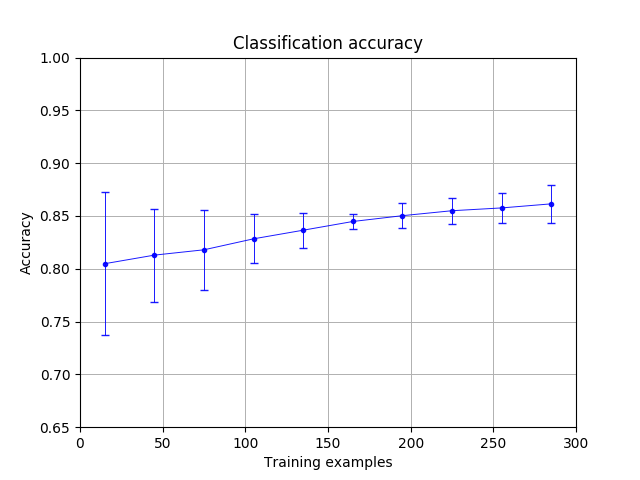
The algorithm’s sampling rate can be chosen; since each event is represented with only 4 data points in our study, we use all 4 data points to characterize every event. 50 runs of the TDA-based classifier were conducted to obtain the average classification accuracy (the ratio of the number of true positives to the total number of predictions made). The results are presented in Figure 1. The TDA-based classifier has 80.5% accuracy when using 15 training examples, increasing to 86.2% with 285 training examples. In general, the classifier seems to be more stable (the classification accuracy deviates less among 50 runs) when increasing the number of training examples.
可以选择算法的采样率。 由于在我们的研究中每个事件仅用4个数据点表示,因此我们使用所有4个数据点来表征每个事件。 进行了50次基于TDA的分类器,以获取平均分类精度(真实阳性数与预测总数之比)。 结果显示在图1中。当使用15个训练示例时,基于TDA的分类器的准确度为80.5%,使用285个训练示例时提高到86.2%。 通常,当增加训练示例的数量时,分类器似乎更稳定(分类准确度在50次运行中偏差较小)。
码: (Code:)
The code is available here: https://zenodo.org/badge/latestdoi/208948304
可以在这里找到代码: https : //zenodo.org/badge/latestdoi/208948304
翻译自: https://towardsdatascience.com/using-machine-learning-in-solar-physics-22f83a0c479c
机器学习 物理引擎


 3520
3520


 被折叠的 条评论
为什么被折叠?
被折叠的 条评论
为什么被折叠?
 到【灌水乐园】发言


