机器学习:分类_机器学习基础：K最近邻居分类

机器学习:分类

In the previous stories, I had given an explanation of the program for implementation of various Regression models. Also, I had described the implementation of the Logistic Regression model. In this article, we shall see the algorithm of the K-Nearest Neighbors or KNN Classification along with a simple example.

在先前的故事中 ，我已经解释了用于实现各种回归模型的程序。 另外，我已经描述了Logistic回归模型的实现。 在本文中，我们将看到K最近邻算法或KNN分类算法以及一个简单示例。

KNN分类概述 (Overview of KNN Classification)

The K-Nearest Neighbors or KNN Classification is a simple and easy to implement, supervised machine learning algorithm that is used mostly for classification problems.

K最近邻或KNN分类是一种简单且易于实现的，受监督的机器学习算法，主要用于分类问题。

Let us understand this algorithm with a very simple example. Suppose there are two classes represented by Rectangles and Triangles. If we want to add a new shape (Diamond) to any one of the classes, then we can implement the KNN Classification model.

让我们通过一个非常简单的示例来了解该算法。 假设有两个用矩形和三角形表示的类。 如果要向任何一个类添加新的形状(钻石)，则可以实现KNN分类模型。

In this model, we have to choose the number of nearest neighbors (N). Here, as we have chosen N=4, the new data point calculates the distance between each of the points and draws a circular region around its nearest 4 neighbors ( as N=4). In this problem as all the four nearest neighbors lie in the Class 1 (Rectangles), the new data point (Diamond) is also assigned as a Class 1 data point.

在此模型中，我们必须选择最近邻居的数量(N)。 在这里，由于我们选择了N = 4，因此新数据点将计算每个点之间的距离，并在其最近的4个邻居周围绘制一个圆形区域(当N = 4时)。 在此问题中，由于四个最近的邻居都位于Class 1(矩形)中，因此新数据点(Diamond)也被分配为Class 1数据点。

In this way, we can alter the parameter, N with various values and choose the most accurate value for the model by a trial and error basis, also avoiding over-fitting and high loss.

这样，我们可以通过反复试验改变参数N的值，并为模型选择最准确的值，从而避免过拟合和高损失。

In this way, we can implement the KNN Classification algorithm. Let us now move to its implementation with a real world example in the next section.

这样，我们可以实现KNN分类算法。 现在，让我们在下一部分中以一个真实的示例转到其实现。

问题分析 (Problem Analysis)

To apply the KNN Classification model in practical use, I am using the same dataset used in building the Logistic Regression model. In this, we DMV Test dataset which has three columns. The first two columns consist of the two DMV written tests (DMV_Test_1 and DMV_Test_2) which are the independent variables and the last column consists of the dependent variable, Results which denote that the driver has got the license (1) or not (0).

为了在实际应用中应用KNN分类模型，我使用的是用于构建Logistic回归模型的相同数据集。 在这里，我们有三列的DMV Test数据集。 前两列包含两个DMV书面测试( DMV_Test_1和DMV_Test_2 )，它们是自变量，最后一列包含因变量， 结果表示驱动程序已获得许可证(1)或没有获得许可证(0)。

In this, we have to build a KNN Classification model using this data to predict if a driver who has taken the two DMV written tests will get the license or not using those marks obtained in their written tests and classify the results.

在这种情况下，我们必须使用此数据构建KNN分类模型，以预测已参加两次DMV笔试的驾驶员是否会使用在其笔试中获得的那些标记来获得驾照，然后对结果进行分类。

步骤1：导入库 (Step 1: Importing the Libraries)

As always, the first step will always include importing the libraries which are the NumPy, Pandas and the Matplotlib.

与往常一样，第一步将始终包括导入NumPy，Pandas和Matplotlib库。

import numpy as np
import matplotlib.pyplot as plt
import pandas as pd

步骤2：导入数据集 (Step 2: Importing the dataset)

In this step, we shall get the dataset from my GitHub repository as “DMVWrittenTests.csv”. The variable X will store the two “DMV Tests ”and the variable Y will store the final output as “Results”. The dataset.head(5)is used to visualize the first 5 rows of the data.

在这一步中，我们将从GitHub存储库中获取数据集，名称为“ DMVWrittenTests.csv”。 变量X将存储两个“ DMV测试 ”，变量Y将最终输出存储为“ 结果 ” 。 dataset.head(5)用于可视化数据的前5行。

dataset = pd.read_csv('https://raw.githubusercontent.com/mk-gurucharan/Classification/master/DMVWrittenTests.csv')X = dataset.iloc[:, [0, 1]].values
y = dataset.iloc[:, 2].valuesdataset.head(5)>>
DMV_Test_1   DMV_Test_2   Results
34.623660    78.024693    0
30.286711    43.894998    0
35.847409    72.902198    0
60.182599    86.308552    1
79.032736    75.344376    1

步骤3：将资料集分为训练集和测试集 (Step 3: Splitting the dataset into the Training set and Test set)

In this step, we have to split the dataset into the Training set, on which the Logistic Regression model will be trained and the Test set, on which the trained model will be applied to classify the results. In this the test_size=0.25 denotes that 25% of the data will be kept as the Test set and the remaining 75% will be used for training as the Training set.

在这一步中，我们必须将数据集分为训练集和测试集，训练集将在该训练集上训练逻辑回归模型，测试集将在训练集上应用训练后的模型对结果进行分类。 在这种情况下， test_size=0.25表示将保留25％的数据作为测试集，而将剩余的75 ％的数据用作培训集 。

from sklearn.model_selection import train_test_split
X_train, X_test, y_train, y_test = train_test_split(X, y, test_size = 0.25)

步骤4：功能缩放 (Step 4: Feature Scaling)

This is an additional step that is used to normalize the data within a particular range. It also aids in speeding up the calculations. As the data is widely varying, we use this function to limit the range of the data within a small limit ( -2,2). For example, the score 62.0730638 is normalized to -0.21231162 and the score 96.51142588 is normalized to 1.55187648. In this way, the scores of X_train and X_test are normalized to a smaller range.

这是一个附加步骤，用于对特定范围内的数据进行规范化。 它还有助于加快计算速度。 由于数据变化很大，我们使用此功能将数据范围限制在很小的限制(-2,2)内。 例如，将分数62.0730638标准化为-0.21231162，将分数96.51142588标准化为1.55187648。 这样，将X_train和X_test的分数归一化为较小的范围。

from sklearn.preprocessing import StandardScaler
sc = StandardScaler()
X_train = sc.fit_transform(X_train)
X_test = sc.transform(X_test)

步骤5：在训练集上训练KNN分类模型 (Step 5: Training the KNN Classification model on the Training Set)

In this step, the class KNeighborsClassifier is imported and is assigned to the variable “classifier”. The classifier.fit() function is fitted with X_train and Y_train on which the model will be trained.

在此步骤中，将导入类KNeighborsClassifier并将其分配给变量“ classifier” 。 classifier.fit()函数配有X_train和Y_train ，将在其上训练模型。

from sklearn.neighbors import KNeighborsClassifier
classifier = KNeighborsClassifier(n_neighbors = 5, metric = 'minkowski', p = 2)
classifier.fit(X_train, y_train)

步骤6：预测测试集结果 (Step 6: Predicting the Test set results)

In this step, the classifier.predict() function is used to predict the values for the Test set and the values are stored to the variable y_pred.

在此步骤中， classifier.predict()函数用于预测测试集的值，并将这些值存储到变量y_pred.

y_pred = classifier.predict(X_test) 
y_pred

步骤7：混淆矩阵和准确性 (Step 7: Confusion Matrix and Accuracy)

This is a step that is mostly used in classification techniques. In this, we see the Accuracy of the trained model and plot the confusion matrix.

这是分类技术中最常用的步骤。 在此，我们看到了训练模型的准确性，并绘制了混淆矩阵。

The confusion matrix is a table that is used to show the number of correct and incorrect predictions on a classification problem when the real values of the Test Set are known. It is of the format

混淆矩阵是一个表，用于在已知测试集的实际值时显示有关分类问题的正确和不正确预测的数量。 它的格式

Source — Self

来源—自我

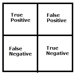
The True values are the number of correct predictions made.

True值是做出正确预测的次数。

from sklearn.metrics import confusion_matrix
cm = confusion_matrix(y_test, y_pred)from sklearn.metrics import accuracy_score 
print ("Accuracy : ", accuracy_score(y_test, y_pred))
cm>>Accuracy :  0.92>>array([[11,  1],
       [ 1, 12]])

From the above confusion matrix, we infer that, out of 25 test set data, 23 were correctly classified and 2 were incorrectly classified which is little better than the Logistic Regression model.

从上面的混淆矩阵中，我们推断出，在25个测试集数据中，有23个被正确分类，而2个被错误分类，这比Logistic回归模型好一点。

步骤8：将实际值与预测值进行比较 (Step 8: Comparing the Real Values with Predicted Values)

In this step, a Pandas DataFrame is created to compare the classified values of both the original Test set (y_test) and the predicted results (y_pred).

在此步骤中，将创建一个Pandas DataFrame来比较原始测试集( y_test )和预测结果( y_pred )的分类值。

df = pd.DataFrame({'Real Values':y_test, 'Predicted Values':y_pred})
df>> 
Real Values   Predicted Values
0             0
0             1
1             1
0             0
0             0
1             1
1             1
0             0
0             0
1             1
0             0
1             0
1             1
1             1
0             0
0             0
0             0
1             1
1             1
1             1
1             1
0             0
1             1
1             1
0             0

Though this visualization may not be of much use as it was with Regression, from this, we can see that the model is able to classify the test set values with a decent accuracy of 92% as calculated above.

尽管这种可视化可能不像使用回归那样有用，但是从中我们可以看到，该模型能够以如上计算的92％的准确度对测试集值进行分类。

步骤9：可视化结果 (Step 9: Visualizing the Results)

In this last step, we visualize the results of the KNN Classification model on a graph that is plotted along with the two regions.

在这最后一步中，我们在与两个区域一起绘制的图形上可视化KNN分类模型的结果。

from matplotlib.colors import ListedColormap
X_set, y_set = X_test, y_test
X1, X2 = np.meshgrid(np.arange(start = X_set[:, 0].min() - 1, stop = X_set[:, 0].max() + 1, step = 0.01),
                     np.arange(start = X_set[:, 1].min() - 1, stop = X_set[:, 1].max() + 1, step = 0.01))
plt.contourf(X1, X2, classifier.predict(np.array([X1.ravel(), X2.ravel()]).T).reshape(X1.shape),
             alpha = 0.75, cmap = ListedColormap(('red', 'green')))
plt.xlim(X1.min(), X1.max())
plt.ylim(X2.min(), X2.max())
for i, j in enumerate(np.unique(y_set)):
    plt.scatter(X_set[y_set == j, 0], X_set[y_set == j, 1],
                c = ListedColormap(('red', 'green'))(i), label = j)
plt.title('KNN Classification')
plt.xlabel('DMV_Test_1')
plt.ylabel('DMV_Test_2')
plt.legend()
plt.show()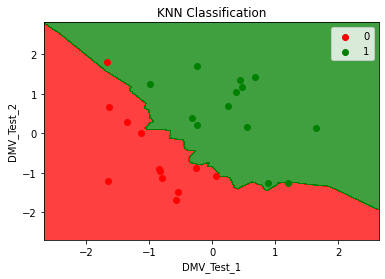

KNN Classification

KNN分类

In this graph, the value 1 (i.e, Yes) is plotted in “Red” color and the value 0 (i.e, No) is plotted in “Green” color. The KNN Classification model separates the two regions. It is not linear as the Logistic Regression model. Thus, any data with the two data points (DMV_Test_1 and DMV_Test_2) given, can be plotted on the graph and depending upon which region if falls in, the result (Getting the Driver’s License) can be classified as Yes or No.

在该图中，值1(即“是”)以“ 红色 ”颜色绘制，而值0(即“否”)以“ 绿色 ”颜色绘制。 KNN分类模型将两个区域分开。 它与Logistic回归模型不是线性的。 因此，具有给定两个数据点(DMV_Test_1和DMV_Test_2)的任何数据都可以绘制在图形上，并且根据所处的区域而定，结果(获得驾驶执照)可以分类为是或否。

As calculated above, we can see that there are two values in the test set, one on each region that are wrongly classified.

如上计算，我们可以看到测试集中有两个值，每个区域一个值被错误分类。

结论— (Conclusion —)

Thus in this story, we have successfully been able to build a KNN Classification Model that is able to predict if a person is able to get the driving license from their written examinations and visualize the results.

因此，在这个故事中，我们已经成功地建立了一个KNN分类模型，该模型能够预测一个人是否能够通过笔试获得驾照并将结果可视化。

I am also attaching the link to my GitHub repository where you can download this Google Colab notebook and the data files for your reference.

我还将链接附加到我的GitHub存储库中，您可以在其中下载此Google Colab笔记本和数据文件以供参考。

You can also find the explanation of the program for other Classification models below:

您还可以在下面找到其他分类模型的程序说明：

• Logistic Regression

  逻辑回归

• K-Nearest Neighbours (KNN) Classification
  K最近邻居(KNN)分类
• Support Vector Machine (SVM) Classification (Coming Soon)
  支持向量机(SVM)分类(即将推出)
• Naive Bayes Classification (Coming Soon)
  朴素贝叶斯分类(即将推出)
• Random Forest Classification (Coming Soon)
  随机森林分类(即将推出)

We will come across the more complex models of Regression, Classification and Clustering in the upcoming articles. Till then, Happy Machine Learning!

在接下来的文章中，我们将介绍更复杂的回归，分类和聚类模型。 到那时，快乐机器学习！

翻译自: https://towardsdatascience.com/machine-learning-basics-k-nearest-neighbors-classification-6c1e0b209542

机器学习:分类