从头开始vue创建项目_从头开始使用JavaScript创建深度学习库（第2部分）

从头开始vue创建项目

In part 1 of this tutorial series, we dove deep into some of the nitty-gritty aspects and foundations of implementing our own deep learning library in JavaScript

在本教程系列的第1部分中 ，我们深入探讨了用JavaScript实现我们自己的深度学习库的一些实质性方面和基础。

We also implemented some basic math operations on single value functions—with this, we were able to see how automatic gradient calculation works, and we also learned the idea behind the static graph.

我们还在单值函数上实现了一些基本的数学运算-借此，我们可以看到自动梯度计算的工作原理，并且还了解了静态图的思想。

In part 2, we’ll discuss how to implement tensors and some basic operations needed to create a simple neural network.

在第2部分中，我们将讨论如何实现张量以及创建简单神经网络所需的一些基本操作。

目标 (Goals)

• Understanding tensors in JavaScript
  了解JavaScript中的张量
• Convert single-value operations (add and multi) to tensor operations
  将单值运算(加和乘)转换为张量运算
• Implement linear layers, a ReLU activation function, and a softmax function
  实现线性层，ReLU激活功能和softmax功能

了解张量 (Understanding Tensors)

A tensor may be represented as a (potentially multidimensional) array (although a multidimensional array is not necessarily a representation of a tensor, as discussed below with regard to holors). Just as a vector in an n-dimensional space is represented by a one-dimensional array with n components………. Wikipedia

张量可以表示为(可能是多维的)数组(尽管多维数组不一定是张量的表示， 如下文有关整体的讨论 )。 就像n 维空间中的向量由具有n个分量的一维数组表示一样…………。 维基百科

In simple terms, just think of tensors as objects that can take in a vector, matrix, or even a multidimensional matrix.

简而言之，将张量视为可以接受矢量，矩阵甚至多维矩阵的对象。

It was much easier for us to experiment with single-value functions in JavaScript, but it becomes more difficult with tensors, since in general JavaScript does not have an attribute that makes math operations easier, like those in Python.

对于我们来说，使用JavaScript进行单值函数的实验要容易得多，但是使用张量则变得更加困难，因为通常而言，JavaScript不像Python中那样具有使数学运算更容易的属性。

For example, Python classes have a dunder attribute (i.e. magic methods) and the like that simplify these operations:

例如，Python类具有dunder属性(即magic方法 )等可简化这些操作的类：

• __add__ to add two class with the same identity property

  __add__添加具有相同标识属性的两个类

• __sub__ to subtract

  __sub__减去

• __mul__ to multiply

  __mul__相乘

• __div___ to divide

  __div___划分

These dunder methods makes it easier to implement tensors like this in Python:

这些dunder方法使在Python中更容易实现这样的张量：

class Tensors():     def __init__(value_list):
          self.data = value_list     def __add__(self, tensor_class):
          return self.data + tensor_class.data     def __sub__(self,tensor_class):
           return self.data - tensor_class.data

With this, it’s easier to create tensor and perform normal tensor operations.

有了它，创建张量和执行正常的张量操作变得更加容易。

In JavaScript, we don’t have such a luxury, but it’s still possible. For this tutorial, we’ll be creating a class for each of those aforementioned math operations.

在JavaScript中，我们没有这么奢侈的东西，但是仍然有可能。 在本教程中，我们将为上述每个数学运算创建一个类。

First, let’s talk about the tensor input. In Python, we structure input tensors like this:

首先，让我们谈谈张量输入。 在Python中，我们像这样构造输入张量：

array([
    [2, 3, 4],
    [5, 6, 7],
    [8, 9,10]
])

While I was trying to implement tensors in JavaScript (during experimentation), the first mistakes I made earlier was, thinking of a tensor as a nested list—like the way they’re implemented in Python.

当我尝试在JavaScript中实现张量时(在实验过程中)，我先前犯的第一个错误是将张量视为嵌套列表，就像它们在Python中的实现方式一样。

This made it difficult to implement some operations involving some technical overhead of using for-loops

这使得难以执行一些涉及使用for循环的技术开销的操作

And for me, I like to build an intuition of how things work and then follow up from there, but using the normal tensor input was not helping.

对我来说，我想对事物如何运作建立直觉，然后从那里进行跟进，但是使用正常的张量输入无济于事。

But after studying the work of Andrej Karpathy on ConvNet.js, I found that I can think of matrices/tensors in different ways.

但研究工作后， 安德烈Karpathy上ConvNet.js ，我发现，我能想到的方式不同矩阵/张量。

The best form was to think of it as a flattened matrix. With this idea, Andrej was able to implement convolutional layers in JavaScript.

最好的形式是将其视为扁平矩阵。 有了这个想法，Andrej能够在JavaScript中实现卷积层。

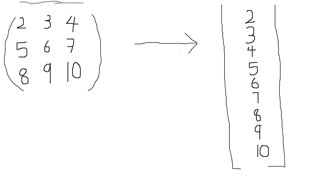
From the above image, you can see how a nested list (matrix) flattens out. The main question is, how do we access the matrix row and columns in the order in which they were created in the original matrix.

从上面的图像中，您可以看到嵌套列表(矩阵)如何展平。 主要问题是，如何按原始矩阵中创建矩阵的顺序访问矩阵的行和列。

Let’s first create the Tensor object and its properties:

首先创建Tensor对象及其属性：

In the Tensor object, n stands for the number of rows and d stands for the number of columns—it also represents depth in the case of 3dim. And we set the outgoing matrix and its gradient to zero, using the zeros utility function.

在Tensor对象中， n代表行数， d代表列数，在3dim的情况下，它还表示depth 。 然后，我们使用zeros实用程序功能将输出矩阵及其梯度设置为零。

Our main focus now should be on the get and set properties—these show how the tensor value is accessed. Let’s illustrate this with a basic example:

现在，我们的主要重点应该放在get和set属性上，这些属性显示了如何访问张量值。 让我们用一个基本的例子来说明这一点：

//given a matrix 3 x 3
[[2, 3, 4],
 [5, 6, 7],
 [8, 9, 10]]

Our aim will be to reduce the above matrix to:

我们的目标是将上述矩阵简化为：

[2,3,4,5,6,7,8,9,10]

To access this array, we multiply the number of columns by the rows and then move in the direction of the column.

要访问此数组，我们将列数乘以行，然后向列方向移动。

(col * row) + col_i

Now let’s see how it works:

现在让我们看看它是如何工作的：

//for 3 x 3 matrix we have n_col = 3, n_rows = 3
//hence the length of the matrix is 9//to access any of the value, let say we want to access all values for row 0//values for row 0
3 * 0 + 0 = 0
3 * 0 + 1 = 1
3 * 0 + 2 = 2   // this are the index of the value of row 0//value for row 1
3 * 1 + 0 = 3
3 * 1 + 1 = 4
3 * 1 + 2 = 5//value for row 3
3 * 2 + 0 = 6
3 * 2 + 1 = 7
3 * 2 + 2 = 8

The main essence of the illustration above is to help show how we access values at an index in the tensors.

上面插图的主要实质是帮助说明我们如何访问张量索引处的值。

Let’s experiment with this in code, creating a 3 X 3 tensor:

让我们在代码中进行实验，创建一个3 X 3张量：

array([[2,3,4],
       [5,6,7],
       [8,9,10])

And don’t forget, our input will not be in the above format. It has to be flattened:

别忘了，我们的输入将不会采用上述格式。 必须将其展平：

[2,3,4,5,6,7,8,9,10]

Note: I could abstract this from the user of the code and let them input the normal NumPy array format and then flatten the input array internally, but for the case of this tutorial, I decided to let it be for clearer understanding.

注意 ：我可以从代码的用户那里抽象出来，让他们输入正常的NumPy数组格式，然后在内部展平输入数组，但是对于本教程而言，我决定让它更清晰地理解。

So in code, this is how this looks:

因此，在代码中，这是这样的：

From the code above, we were able to get the value at row 1 and column 2.

从上面的代码中，我们能够获得第1行和第2列的值。

Let’s also try to change the value at row 1 column 2:

让我们也尽量在行更改值1列2 ：

This method will really help us perform easy dot-products.

这种方法确实可以帮助我们完成简单的点积运算。

Since we’ve created the Tensor object for a 2-dimensional array, let’s convert our former Add operation to a 2-dimensional one:

由于我们已经为二维数组创建了Tensor对象，因此让我们将以前的Add操作转换为二维数组：

In this new Add class, I did not use gradv to store the incoming gradient, but it’s now represented with dout.

在这个新的Add类中，我没有使用gradv来存储输入的渐变，但是现在用dout表示了。

For the addition operation, instead of using the get method in in the Tensor class, we access the tensor just like a normal JavaScript array: this.items.out[i] = x.out[i] + y.out[i];

对于加法运算，我们不像在Tensor类中使用get方法那样，而是像普通JavaScript数组一样访问张量： this.items.out[i] = x.out[i] + y.out[i];

We did this since the two inputs must have the same length:

我们这样做是因为两个输入必须具有相同的长度：

The dot operation is done in the above code, as shown here:

点操作在上面的代码中完成，如下所示：

dot += this.x.get(i,k) * this.y.get(k,j);

In the dot operation, if we have two matrices of A(2X3) and B(3X4), the output of the dot operation will be 2X4.

在点运算中，如果我们有两个矩阵A(2X3)和B(3X4)，则点运算的输出将为2X4。

This is done by first looping through the column of each row in matrix A and then multiplying and adding each element by the row of each column in matrix B.

这是通过首先循环遍历矩阵A中每一行的列，然后将每个元素乘以矩阵B中每一列的行来完成的。

And for backpropagation, don’t forget that the derivative of a multiplying function (of a two-value input) with respect to one of its inputs is equal to the other input.

对于反向传播，请不要忘记(两个值输入的)乘法函数相对于它的一个输入的导数等于另一个输入。

For dot products, this will be quite different, but we’ll go into more detail about that later.

对于点产品，这将大不相同，但是稍后我们将对此进行更详细的介绍。

this.x.dout[this.x.d*i+k] += this.y.out[this.y.d*k+j] * b;

In the code snippet above, the derivative value is multiplied by the incoming gradient b.

在上面的代码段中，导数值乘以输入梯度b 。

Let’s try a simple example: A dot operation between two matrices of shape 2x3 and 3X2.

让我们尝试一个简单的示例：两个形状为2x3和3X2的矩阵之间的点运算。

Note: One rule of dot product is that the column size of the first matrix must be equal to the row size of the second matrix.

注意 ：点积的一条规则是，第一个矩阵的列大小必须等于第二个矩阵的行大小。

matrix A (2X3): [[6,5,4],
                 [3,2,1]]matrix B (3X2): [[1,2],
                 [3,4],
                 [5,6]]

If we find the dot product between two matrices, we should expect an output matrix of shape (2X2).

如果我们找到两个矩阵之间的点积，则应该期望得到形状为(2X2)的输出矩阵。

The dot product between the two matrices will look like this:

这两个矩阵之间的点积如下所示：

A * B[(6*1+5*3+4*5), (6*2+5*4+4*6)] = [41,56][(3*1+2*3+1*5), (3*2+2*4+1*6)] = [14,20]

Hence, the output matrix from the above operation is:

因此，上述操作的输出矩阵为：

[[41,56],
 [14,20]]

With this, let’s try it out with the matmul class:

有了这个，让我们尝试一下matmul类：

Using the code above, we get the same output calculated before:

使用上面的代码，我们得到之前计算出的相同输出：

[41,54,14,20]

Now let’s perform backpropagation for the above operation.

现在让我们对上述操作进行反向传播。

If you’ll recall…

如果您还记得...

And for backpropagation, don’t forget that the derivative of a multiplying function (of a two-value input) with respect to one of its inputs is equal to the other input.

对于反向传播，请不要忘记(两个值输入的)乘法函数相对于它的一个输入的导数等于另一个输入。

For the dot product, the same fact still remains. But since we’re dealing with a tensor, the derivative of the function f(x,y) = xy with respect to its input is given as:

对于点积，仍然存在相同的事实。 但是由于我们要处理张量，因此函数f(x，y)= xy相对于其输入的导数为：

df/dy = transpose of x and df/dx= transpose of y

df/dy = transpose of x and df/dx= transpose of y

But don’t forget, we’re dealing with gradient inflow from the top of the graph downward, i.e the matmul operation will be receiving some gradient.

但是请不要忘记，我们正在处理从图的顶部开始向下的梯度流入，即matmul操作将接收一些梯度。

Therefore, the derivative df/dy = gradient_in_flow * transpose of x

因此，导数df/dy = gradient_in_flow * transpose of x

Now, to calculate the backprop for the code above, let’s assume there’s a dummy gradient inflow, which is a derivative of a function by itself df/df.

现在，要计算上面代码的反向传播，我们假设有一个虚拟梯度流入，它是函数本身df / df的派生。

The gradient will be of the same shape as the computed output from the matmul operation, which is (2X2).

梯度的形状与matmul运算的计算结果(2X2)相同。

Now to calculate the backprop for the tensor variable a:

现在计算张量变量a的反向传播：

gradient_inflow = [[1,1],
                   [1,1]]df/da = gradient_inflow * b_transpose

To get b transpose, we invert the matrix axis:

为了使b转置，我们反转矩阵轴：

b = [[1,2],
     [3,4],
     [5,6]]b_transpose = [[1,3,5],
               [2,4,6]]

Hence, df/da is given as:

因此，df / da为：

[[1,1],    *   [[1,3,5],
 [1,1]]        [2,4,6]]//just like we did the dot product before
[(1*1+1*2), (1*3+1*4), (1*5+1*6)] = [3,7,11]
[(1*1+1*2), (1*3+1*4), (1*5+1*6)] = [3,7,11]

The gradient df/da as a shape (2X3), which is also the same shape as tensor A. The gradient of a tensor must be of the same shape as the tensor itself.

梯度df / da的形状为(2X3)，也与张量A的形状相同。张量的梯度必须与张量本身的形状相同。

Now let’s take a look at the code to implement this:

现在让我们看一下实现此代码：

Since we’ve been able to create the Add and matmul objects, we now have full access to create a linear layer.

由于我们已经能够创建Add和matmul对象，因此我们现在拥有创建线性层的完全权限。

线性层 (Linear Layer)

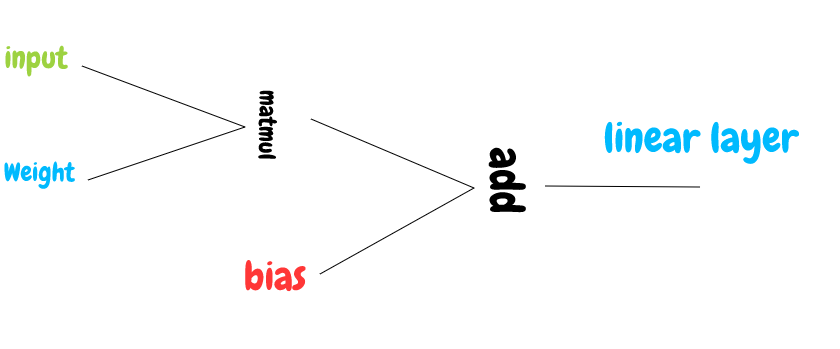
A linear layer is made up of simple math operations; addition and matmul.

线性层由简单的数学运算组成； 除了和matmul。

The function for a linear layer is given as F(X) = x*W + b

线性层的函数为F(X) = x*W + b

Let’s go ahead and implement a linear layer:

让我们继续实施线性层：

The Linear layer object takes in the input dimension and the output dimension, which are used to initialize the weight and the bias.

Linear图层对象接受输入尺寸和输出尺寸，这些尺寸用于初始化权重和偏差。

this.W = new Tensor(in_dim,out_dim,true).randn(0,0.88); // initialize the weight        this.b = new Tensor(out_dim,1,true).randn(0,0.88); // initialoze bia

The weight and bias are initialized with a random variable generated from a Gaussian distribution with a mean of 0 and a standard deviation of 0.88. They are trainable parameters

权重和偏差使用从高斯分布生成的随机变量初始化，平均值为0，标准偏差为0.88。 它们是可训练的参数

The forward pass for the linear layer involves the use of the matmul and Add objects.

线性层的前向传递涉及使用matmul和Add对象。

this.mult = new Matmul(x,this.W)            
this.items = new add(this.mult,this.b);

And backprop is done using the backward function:

反向传播是使用backward功能完成的：

backward: function(){                    
      this.items.grad(this.dout);                                this.items.backward(); //backprop accross the chain        
},

From the code above, you can now see that we don’t need to define backpropagation explicitly. Instead, this.items.backward() is used to do the magic.

从上面的代码中，您现在可以看到我们不需要显式定义反向传播。 而是使用this.items.backward()做魔术。

Specifically, this.items.backward() is used to call operations associated with the operator. For example, the forward operation is like this matmul → add , but when this.items.backward() is called the operation looks like this add → matmul.

具体来说， this.items.backward()用于调用与运算符关联的操作。 例如，前向操作类似于此matmul → add ，但是在this.items.backward()时，操作类似于此add → matmul 。

That is, we calculate the derivative for the add operation, and then pass in the gradient generated from the add operation to its input.

也就是说，我们计算add运算的导数，然后将add运算生成的梯度传递到其输入。

The input to the add operation is matmul and bias , and the gradient passed down is used to calculate the derivative for matmul with respects to its input x and weight w.

add运算的输入为matmul和bias ，向下传递的梯度用于计算matmul于其输入x和权重w 。

I hope now you can see the chain:

我希望现在您可以看到链条：

linear layer computational graph

线性层计算图

Let’s try an example to test our linear layer. We’ll be setting the weight to a more defined set of numbers instead of random ones.

让我们尝试一个示例来测试我们的线性层。 我们将权重设置为一组更定义的数字，而不是随机数。

With this, we can see the gradient inflow and see if the basic operation is done correctly:

这样，我们可以看到梯度流入，并查看基本操作是否正确完成：

If you try to investigate the gradient a.dout , linear.W.dout , linear.b.out , you’ll see that their values as produced by the code above are correct.

如果您尝试研究梯度a.dout ， linear.W.dout ， linear.b.out ，那么您会发现上面的代码生成的它们的值是正确的。

Before we moved on to implement our activation functions, let’s revisit the forward method of the linear layer.

在继续实现激活功能之前，让我们重新回顾线性层的forward方法。

forward : function(x){                
   this.mult = new Matmul(x,this.W)            
   this.items = new add(this.mult,this.b);
   this.n = this.mult.n;           
   this.d = this.mult.d;           
   this.out = this.items.out;            
   this.dout = this.items.dout;                               return this;       
 },

The forward method returns this —in JavaScript, this is a very important keyword.

forward方法返回this -在JavaScript中， this是一个非常重要的关键字。

this refers to the owner of the method. With this keyword, the forwardpass variable is able to retain the property of the linear layer. Also because of this keyword, we can run backpropagation with the forwardPass, using forwardPass.backward(), and we’ll still see the changes reflected.

this是指方法的所有者。 使用此关键字， forwardpass变量能够保留线性层的属性。 同样由于这个关键字，我们可以使用forwardPass.backward()与forwardPass进行反向传播，并且仍然会看到更改。

this also makes it possible to build the graph-like structure, similar to the chainer structure in libraries like jQuery. This structure then makes it possible to pass a linear layer to another layer, while still being able to calculate the derivative down the line:

this也使构建类似于jQuery之类的链接器结构的图状结构成为可能。 然后，此结构使将线性层传递到另一层成为可能，同时仍然能够沿线计算导数：

linear_layer1 = new Linear(2,3,true)
linear_layer2 = new Linear(3,2,true)linear1_output = linear_layer1.forward(x)
linear2_output = linear_layer2.forward(linear1_output)linea2_output.backward()

ReLu激活功能 (ReLu Activation Function)

I’m working under the assumption that you have at least a basic understanding of activation functions like the ones we’ll be working with. But just in case, I’ll also provide a quick overview

我正在假设您至少对激活功能(如我们将要使用的激活功能)有基本的了解。 但以防万一，我还将提供快速概述

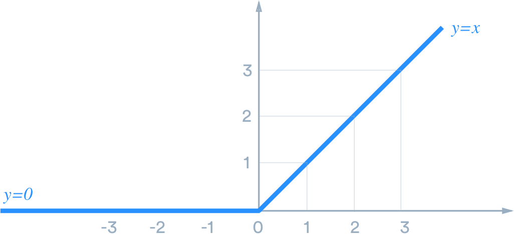
ReLU is an activation function, which helps us prevent gradient saturation.

ReLU是激活功能，可帮助我们防止梯度饱和。

And in general, activation functions are used to increase an ML model’s capacity by converting the linear layer to a non-linear layer.

通常，激活函数通过将线性层转换为非线性层来增加ML模型的容量。

The ReLU activation function is represented by f(x) = max(0,x)

ReLU激活函数由f(x)= max(0，x)表示

ReLU derivative

ReLU衍生物

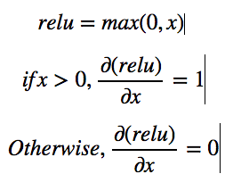
The above image shows how to find the derivative of ReLU with respect to its input.

上图显示了如何找到ReLU关于其输入的导数。

But for our design, remember that there will always be a gradient inflow. hence for if x> 0, dL/dx = d(relu)/dx * dL/d(relu), if we assume that the gradient is coming from function L .

但是对于我们的设计，请记住始终会有梯度流入。 因此， if x> 0 ，则dL/dx = d(relu)/dx * dL/d(relu) ，如果我们假设梯度来自函数L

Hence for if x> 0, dL/dx = 1 * dL/d(relu).

因此， if x> 0 ，则dL/dx = 1 * dL/d(relu) 。

The implementation of ReLU, then, looks like this:

那么，ReLU的实现如下所示：

Let’s try implementing this with code:

让我们尝试使用代码来实现：

let a = new autograd.Tensor(1,5,true)a.setFrom([1,2,3,-4,-5])let relu = new autograd.ReLU()let relu_pass = relu.forward(a)console.log(relu_pass.out);//output
[1,2,3,0,0]

Notice that all the operations (Linear, ReLu) are using the same structure. Now let’s do the same for a softmax activation function

请注意，所有操作( Linear ， ReLu )都使用相同的结构。 现在让我们对softmax激活函数进行相同的操作

软最大 (Softmax)

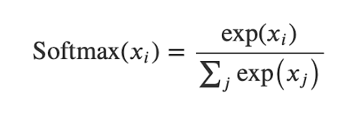
Softmax is also an activation function used at the output layer of neural networks. It’s a probability function in which the total value sums to one.

Softmax也是在神经网络输出层使用的激活函数。 这是一个概率函数，其总和为1。

The implementation:

实现：

In the forward method, while calculating the softmax, we make sure all the data points are subtracted from the maximum value in order to to prevent float number overflow.

在前forward方法中，在计算softmax时，我们确保从最大值中减去所有数据点，以防止浮点数溢出。

Now that we’ve been able to implement a linear layer and ReLU and softmax activation functions, we’re set to create our first simple neural network.

既然我们已经能够实现线性层以及ReLU和softmax激活函数，那么我们就可以创建我们的第一个简单神经网络。

We’re able to create a two-layer neural network. And as you can see from the code snippet , the output of the softmax sums up to one. To calculate backpropagation, we just need to input the index of the correct class to backward method in the softmax function.

我们能够创建一个两层的神经网络。 从代码片段中可以看到，softmax的输出总和为1。 要计算反向传播，我们只需要在softmax函数中向backward方法输入正确类的索引。

Let’s imagine that the neural network is for binary classification, and the correct class is 1. Hence, the code will look like this:

假设神经网络用于二进制分类，正确的分类是1 。 因此，代码将如下所示：

softmax.backward(1)console.log(linear1.dout,linear2.dout)

At this point, it’d be smart to also investigate if the operations are properly done.

此时，最好调查一下操作是否正确完成。

结论 (Conclusion)

That’s all for this part of our tutorial series. Some key points to remember:

这就是我们的教程系列的全部内容。 需要记住的一些关键点：

• this keyword helps us enable the chain property, which is key for creating a computational graph.

  this关键字帮助我们启用链属性，这是创建计算图的关键。

• To implement the whole process for another programming language that does not naturally support numerical operations, you need to understand how to represent tensors in the easiest way.
  要为另一种自然不支持数值运算的编程语言实现整个过程，您需要了解如何以最简单的方式表示张量。
• Each operation has the same basic structure.
  每个操作具有相同的基本结构。

• require_grad helps control gradient flow into a node.

  require_grad帮助控制渐变流向节点的流动。

In the next part, we’ll be implementing a sequential layer, an optimizer and a loss function (cross-entropy) Stay tuned!

在下一部分中，我们将实现顺序层，优化器和损失函数(交叉熵)，敬请期待！

Editor’s Note: Heartbeat is a contributor-driven online publication and community dedicated to exploring the emerging intersection of mobile app development and machine learning. We’re committed to supporting and inspiring developers and engineers from all walks of life.

编者注： 心跳 是由贡献者驱动的在线出版物和社区，致力于探索移动应用程序开发和机器学习的新兴交集。 我们致力于为各行各业的开发人员和工程师提供支持和启发。

Editorially independent, Heartbeat is sponsored and published by Fritz AI, the machine learning platform that helps developers teach devices to see, hear, sense, and think. We pay our contributors, and we don’t sell ads.

Heartbeat在编辑上是独立的，由以下机构赞助和发布 Fritz AI ，一种机器学习平台，可帮助开发人员教设备看，听，感知和思考。 我们向贡献者付款，并且不出售广告。

If you’d like to contribute, head on over to our call for contributors. You can also sign up to receive our weekly newsletters (Deep Learning Weekly and the Fritz AI Newsletter), join us on Slack, and follow Fritz AI on Twitter for all the latest in mobile machine learning.

如果您想做出贡献，请继续我们的 呼吁捐助者 。 您还可以注册以接收我们的每周新闻通讯(《 深度学习每周》 和《 Fritz AI新闻通讯》 )，并加入我们 Slack ，然后继续关注Fritz AI Twitter 提供了有关移动机器学习的所有最新信息。

翻译自: https://heartbeat.fritz.ai/create-a-deep-learning-library-in-javascript-from-scratch-part-2-11fc5e94a8a

从头开始vue创建项目