


sympy表达式简化
Machine learning requires some calculus. Many of the online Machine learning courses don’t always cover the basics of calculus assuming the user already has a foundation. If you are anything like me, you might need a bit of a refresher. Let’s take a look at a few basic calculus concepts and how to write them in your code using SymPy.
机器学习需要一些演算。 假设用户已经具备基础知识,那么许多在线机器学习课程并不总是涵盖微积分的基础知识。 如果您像我一样,则可能需要一些复习。 让我们看一些基本的微积分概念,以及如何使用SymPy在代码中编写它们。
Most of the time, we need calculus to find the derivatives in optimization problems. This helps us to decide whether to increase or decrease weights. Our end goal is to find an extreme point(s) which will be the local minimum or maximum point(s) in a function.
大多数时候,我们需要演算来找到优化问题中的导数。 这有助于我们确定是增加还是减少重量。 我们的最终目标是找到一个极限点,该极限点将成为函数中的局部最小或最大点。
Let’s go through the process of finding an extreme point by taking the following steps.
让我们通过执行以下步骤来完成寻找极端点的过程。
- Installing and learning the basics of Sympy. 安装和学习Sympy的基础知识。
- Finding the slope of a linear function. 求线性函数的斜率。
- Discovering tangent and secant lines. 发现切线和割线。
- Using our slope and tangent line knowledge to find limits. 使用我们的坡度和切线知识来查找极限。
- Understanding what the derivative of a function is. 了解什么是函数的导数。
- Using the derivative to find the extreme point. 使用导数找到极限点。
- Deciding whether the extreme point is a local minimum or a maximum point. 确定极端点是局部最小值还是最大值。
SymPy入门 (Getting Started With SymPy)
SymPy is a Python library that lets you use symbols to compute various mathematic equations. It includes functions to calculate calculus equations. It also includes many other functions for some higher-level mathematics.
SymPy是一个Python库,可让您使用符号来计算各种数学方程式。 它包括计算微积分方程的函数。 它还包括一些用于某些高级数学的其他功能。
Installing SymPy is simple you can find full installation instructions here. If you are already using Anaconda, SymPy is included. With Anacona you can make sure your SymPy is up to date with a simple:
安装SymPy非常简单,您可以在此处找到完整的安装说明。 如果您已经在使用Anaconda,则包括SymPy。 使用Anacona,您可以通过以下简单操作来确保您的SymPy是最新的:
conda update sympyIf you aren’t using Anaconda, pip is a great way to install new Python libraries.
如果您不使用Anaconda,pip是安装新Python库的好方法。
pip install sympySymPy depends on the mpmath library so you’ll need that installed too.
SymPy依赖于mpmath库,因此您也需要安装该库。
conda install mpmath
#or
pip install mpmath
With SymPy we can create variables like we would in a math equation. We need to set these variables as symbols so SymPy knows to treat them differently than regular Python variables. This is simple and accomplished using the symbols() function.
使用SymPy,我们可以像在数学方程式中一样创建变量。 我们需要将这些变量设置为符号,以便SymPy知道与常规Python变量不同的对待方式。 这很简单,可以使用symbol()函数完成。
import sympy
x2, y = sympy.symbols('x2 y')
Now that we have SymPy installed let’s take a step back and look at the foundations of calculus.
现在我们已经安装了SymPy,让我们退后一步,看一下微积分的基础。
线性方程和斜率 (Linear Equations and the Slope)
As mentioned above one of the main reasons we need calculus is to find the extreme point(s). To illustrate this, let’s pretend every year you enter the Annual Potato Cannon Contest. Every year you lose to the terrible Danny MacDougal. This year you hire a coach to help you beat Danny. To beat Danny, the coach needs you to give him three things.
如上所述,我们需要演算的主要原因之一是找到极限点。 为了说明这一点,让我们假装每年参加年度马铃薯大炮竞赛。 每年,您都会输给可怕的丹尼·麦克杜格尔(Danny MacDougal)。 今年,您聘请了一位教练来帮助您击败丹尼。 要击败丹尼,教练需要您给他三件事。
1. When Danny’s potato is at it’s highest point.
1.当丹尼的土豆达到最高点时。
2. How long it takes the potato to get to the highest point.
2.马铃薯到达最高点需要多长时间。
3. The slope of the potato at its highest point.
3.马铃薯在最高点的坡度。
Let’s talk first about the slope.
让我们先谈谈坡度。
If Danny built a magic cannon where the potato ascended forever finding the slope would be easy but there wouldn’t be a maximum height. This type of potato flight path is would be a linear equation like y = 3x + 2 (in y-intercept form).
如果丹尼(Danny)建造了一个神奇的大炮,马铃薯永远登高,发现斜坡很容易,但不会达到最大高度。 这种类型的马铃薯飞行路径将是一个线性方程,例如y = 3x + 2(以y截距的形式)。
We can visualize this linear function potato flight using NumPy and Matplotlib. If you don’t have NumPy and Matplotlib installed the process is like the SymPy insulation above. See here and here for more details.
我们可以使用NumPy和Matplotlib可视化此线性函数马铃薯飞行。 如果没有安装NumPy和Matplotlib,则过程类似于上面的SymPy绝缘。 有关更多详细信息,请参见此处和此处 。
import matplotlib.pyplot as plt
import numpy as np#create 100 values for x ranging from 0 to 6
x = np.linspace(0,6,100)#our linear function
y = 3*x + 2#add some aesthetics to out plot
plt.grid(color='b', linestyle='--', linewidth=.5)
plt.plot(x,y, label="potato flight")
plt.xlim(0, 6)
plt.ylim(0,20)
plt.legend(loc='best')
plt.xlabel("Seconds")
plt.ylabel("Feet(x10)")#show the plot we created
plt.show()
We want to examine the slope so we will add to marks on two random points: (1,5) and (4,14).
我们要检查斜率,因此我们将在两个随机点上添加标记:(1,5)和(4,14)。
plt.plot(1, 5, 'x', color='red')
plt.plot(4, 14, 'x', color='red')
When we have a linear function our slope is constant and we can calculate it by looking at any two points and calculating the change in y divided by the change x. Let’s look at the two points we marked earlier.
当我们有一个线性函数时,我们的斜率是常数,我们可以通过观察任意两个点并计算y的变化除以x的变化来计算它。 让我们看一下前面标记的两点。
In y-intercept form (y = mx + b) the m is always the slope. This checks out from our previous function of y = 3x + 2.
在y截距形式(y = mx + b)中, m始终是斜率。 这从我们以前的y = 3x + 2函数中检出。
土豆必须降下来—非线性函数 (Potatoes Must Come Down — Nonlinear Functions)
The slope of a linear function is easy but the potato must come down. We need a way to calculate a slope that changes with each point. Let’s start by visualizing a more realistic potato flight path.
线性函数的斜率很容易,但是马铃薯必须下降。 我们需要一种方法来计算随每个点变化的斜率。 让我们从可视化更现实的马铃薯飞行路径开始。
Our coach is amazing and he knows the function that represents the flight of the potato is f(x) = -(x²) +4x.
我们的教练很棒,他知道代表土豆飞行的函数是f(x)=-(x²)+ 4x。
Once again let’s visualize this potato flight path with Matplotlib.
再次让我们通过Matplotlib形象地看待这个马铃薯的飞行路线。
x = np.linspace(0,5,100)
y = -(x**2) + 4*xplt.xlim(0, 4.5)
plt.ylim(0,4.5)
plt.xlabel("Seconds")
plt.ylabel("Height in Feet(x10)")
plt.grid(color='b', linestyle='--', linewidth=.5)
plt.plot(x, y, label="potato")
plt.legend(loc='best')plt.show()
From the visualization of the function, we see that in around 2 seconds the potato is at its height of around 40 feet. The graph is helpful but we still need the slope of the maximum height. Plus we need some hard evidence to bring back to the coach. Let’s move forward proving this height and time with calculus.
通过功能的可视化,我们可以看到在大约2秒钟内土豆的高度约为40英尺。 该图很有用,但我们仍然需要最大高度的斜率。 另外,我们需要一些确凿的证据才能带回教练。 让我们继续通过微积分证明这一高度和时间。
正割线 (Secant Lines)
A secant of a curve is a line that intersects the curve at a minimum of two distinct points. When we have nonlinear functions we can still find the slope between two points, or a secant line. Since (2,4) looks like the top of our potato path, let’s look at 2 points on our new nonlinear potato path: (1,3) and (2,4).
曲线的割线是在至少两个不同点处与曲线相交的线。 当我们具有非线性函数时,我们仍然可以找到两点或割线之间的斜率。 由于(2,4)看起来像是马铃薯路径的顶部,因此让我们看一下新的非线性马铃薯路径上的2个点:(1,3)和(2,4)。
#adding this code to our above plot
x2 = np.linspace(1,2,100)
y2 = x2 + 2
plt.plot(x2,y2, color='green')
We can see that the slope from (1,3) and (2,4) is 1. Let’s take this a step further and see what happens when we try to find the slope of just the point(2,4). To do so we need a line that will be able to represent going through one point.
我们可以看到(1,3)和(2,4)的斜率是1。让我们更进一步,看看尝试找到仅点(2,4)的斜率会发生什么。 为此,我们需要一条能够代表经过一个点的线。
切线 (Tangent Lines)
Let’s see what happens to the slope of our lines the closer we get to (2,4). To so we’ll draw a few more secant lines. We’ll keep the endpoint at (2,4) but one line will start at (1.5, 3,75) and the other one at (1.95, 3.9975). This gives us two more secant lines y3 = .5x + 3 and y4 = .05x + 3.9.
让我们看看越接近(2,4),直线斜率会发生什么。 为此,我们将画出更多的割线。 我们将端点保持在(2,4),但一行将从(1.5,3,75)开始,另一行从(1.95,3.9975)开始。 这给了我们另外两条割线y3 = .5x + 3和y4 = .05x + 3.9。

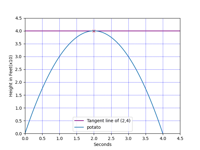
When we finally reach (2,4) as our starting point, a line that forms, which is y = 0x +4. This is the tagent line for (2,4). The tangent line is calculated by solving the limit and plugging it into the y-intercept linear equation. More on the limit in a little bit. Every point in a function has a tangent line, which is how we can calculate the slope for every point in a function.
当我们最终到达(2,4)作为起点时,形成一条直线,即y = 0x +4。 这是(2,4)的标记行。 通过求解极限并将其插入y截距线性方程来计算切线。 一点点就更多了。 函数中的每个点都有一条切线,这就是我们如何计算函数中每个点的斜率。
Remember, our main goal is to find an extreme point, the maximum height of the potato. Extreme points will be when the slope of the tangent line is zero as this will signify when a function changes directions. For instance, let’s look at the slope for the tangent line going through (1,3) and one going through (3,3).
请记住,我们的主要目标是找到一个极限点,即马铃薯的最大高度。 极限点是切线的斜率为零时,因为这表示函数改变方向时。 例如,让我们看一下穿过(1,3)和穿过(3,3)的切线的斜率。

Let’s look at what happened to the slope of the tangent line for these three points.
让我们看看这三个点的切线斜率发生了什么。
point (1,3), the tangent line is y = 2x + 1, slope is 2
点(1,3),切线为y = 2x + 1,斜率为2
point (2,4), the tangent line is y = 0x + 4, slope is 0
点(2,4),切线为y = 0x + 4,斜率为0
point (3,3), the tangent line is y = -2x + 9, slope is -2
点(3,3),切线为y = -2x + 9,斜率为-2
After 0 the slope changes directions. Perfect, we need to find the point or points that have a tangent line with a slope of zero. These points will tell us the maximum or minimum points as the direction of the tangent line slopes will always change after 0.
0后,斜率会改变方向。 完美,我们需要找到切线为零的切线点。 这些点将告诉我们最大或最小点,因为切线斜率的方向将始终在0之后改变。
Great! So we need to find a point on a function where the slope is zero. If only there was a to create a function that would give us the slope of any point in our original function. There is, and that is what the derivative is! Before we jump into derivatives let’s look Limits.
大! 因此,我们需要在函数上找到一个斜率为零的点。 如果只需要创建一个函数,该函数将为我们提供原始函数中任意点的斜率。 存在,这就是派生词! 在开始使用导数之前,让我们看一下Limits 。
限度 (Limits)
Limits allow us to find the slope of a function as it approaches a certain x value. If we are solving the limit as a secant line it’s easy. We plug in our two x values and two y values and we can solve the slope equation. This sort of limit defined. But, we want to find an undefined limit because we want the slope of the tangent line to the point (2,4).
极限使我们能够找到函数接近某个x值时的斜率。 如果我们将极限作为割线来解决,这很容易。 我们插入两个x值和两个y值,就可以求解斜率方程。 定义了这种限制。 但是,我们想要找到一个未定义的极限,因为我们要切线到点(2,4)的斜率。
As we approach (2,4) we need the slope. We can’t get the slope of the secant line from (2,4) to (2,4) because if we plug those numbers into our slope equation we get 0/0. This won’t work because as a math teacher once said: “ There are two things in life you can’t do, nail jello to a wall and divide by zero”. Since we can’t divide by zero we need to find the undefined limit.
当我们接近(2,4)时,我们需要斜率。 我们无法获得从(2,4)到(2,4)的割线的斜率,因为如果将这些数字插入到斜率方程中,则会得到0/0。 这是行不通的,因为正如一位数学老师曾经说过的:“生活中有两件事你做不到,将果冻钉在墙上,然后除以零”。 由于无法将其除以零,因此需要找到未定义的限制。
Limits are solved by plugging our function into the slope equation and factoring it out. We can use our slope formula from before and substitute our point(2,4) for the x1/y1 values and then substitute the f(x) and x for the x2/y2 values. Our limit value is the x value we are approaching, which in this case is 2. Our new slope equation for limit 2 of the function -(x²) +4x is :
通过将我们的函数插入斜率方程并将其分解出来即可解决极限。 我们可以使用之前的斜率公式,将point(2,4)替换为x1 / y1值,然后将f(x)和x替换为x2 / y2值。 我们的极限值为我们接近的x值,在这种情况下为2。我们对函数-(x²)+ 4x的极限2的新斜率方程是:
Our goal is to get rid of the x on the denominator, so let’s expand the -(x²) and cancel out the x on the denominator.
我们的目标是摆脱分母上的x,因此让我们扩展-(x²)并抵消分母上的x。
And now that we have removed the x from the denominator we can put plug 2 back into x.
现在我们已经从分母中删除了x,我们可以将插头2放回x中。
Now that we know how a limit is solved let’s fire up SymPy so we can solve the limit in our code.
现在我们知道如何解决限制,让我们启动SymPy,以便可以在代码中解决限制。
SymPy has a function named limit() which has 3 parameters.
SymPy有一个名为limit()的函数,该函数具有3个参数。
- the function we’re finding the limit for 我们正在寻找极限的功能
- the input variable 输入变量
- the number the input variable is approaching 输入变量接近的数字
Since our limit is undefined we need to subsitute our x and y values as we did above.
由于我们的限制未定义,因此我们需要像上面一样替换x和y值。
import sympy
x2, y = sympy.symbols('x2 y')
#store our substituted function as a y variable
y = (-(x2**2) + 4 * x2 -4) / (x2 -2)
limit = sympy.limit(y, x2, 2)
// 0
Our limit is 0!
我们的限制是0!
衍生品 (Derivatives)
The derivative is a function that will give us the slope of a tangent for any point in our function.
导数是一个函数,它将为我们提供函数中任何点的切线斜率。
Now we understand what the limit and tangent lines are we can head towards our end goal of using derivatives to find the extreme point(s) in the function. The process of finding a function’s derivative is differentiation.
现在我们了解了极限线和切线是什么,我们可以朝最终目标求导,即使用导数在函数中找到极限点。 寻找函数导数的过程是微分 。
Solving the derivative uses some algebra and our slope formula from above. Because we aren’t solving for a specific point we won’t substitute any values. For this example let’s also replace x1 and x2 with the more common form, which is to use x and x +h. This will give us the following formula to solve for the derivative with f′(x) meaning the derivative of the function of x:
从上面使用一些代数和我们的斜率公式来求解导数。 因为我们没有解决特定的问题,所以我们不会替换任何值。 对于此示例,我们还将x1和x2替换为更常见的形式,即使用x和x + h。 这将为我们提供以下公式来求解具有f'(x)的导数,f'(x)表示x函数的导数:
If we plug our function into this we get:
如果将函数插入此函数,则会得到:
We can then solve this similarly to how we solved for the limit. We can also use the power rule to solve to easily find our derivative using the following equation.
然后,我们可以像解决极限一样解决此问题。 我们还可以使用幂规则来求解,以便使用以下公式轻松找到我们的导数。
Using that rule we can see the derivative of our function -(x²) +4x is -2x +4.
使用该规则,我们可以看到函数-(x²)+ 4x的导数是-2x +4 。
Inseatd of going through the steps to find the derivative by hand let’s find the derivative using SymPy.
在完成手动查找导数的步骤之后,让我们使用SymPy查找导数。
SymPy gives us a function called diff() which will perform the differentiation process and returns the derivative.
SymPy给我们提供了一个名为diff()的函数,该函数将执行微分过程并返回导数。
The diff function takes two parameters:
diff函数采用两个参数:
- the function we’re finding the derivative for 我们正在寻找的导数的函数
- the input variable 输入变量
Let’s give this function try using our original function, -(x²) +4x.
让我们尝试使用我们的原始功能-(x²)+ 4x来提供此功能。
# set x as the variable
x = sympy.symbols('x')#help make the out easier to read
sympy.init_printing(use_unicode=True)#enter the our argumnets to th diff funtion
d= sympy.diff(-(x**2) + 4*x, x)#print our derivative
print(d)
//-2*x + 4
Our extreme points in a function will be where our derivative is equal to zero. This is because when the derivative is equal to 0 the direction of the function has changed, as we explored above.
函数的极限点是导数等于零的地方。 这是因为当导数等于0时,函数的方向发生了变化,如我们上面所探讨的。
To find the x value we set our derivative to equal 0 and solve for x, -2x + 4 = 0.
为了找到x值,我们将导数设置为等于0并求解x, -2x + 4 = 0。
This is solved with SymPy by using the function solveset(). Solvest takes two parameters:
这可以通过SymPy通过使用Solveset()函数来解决。 Solvest采用两个参数:
the Eq function which takes two parameters: the equation and the value the equation needs to equal
带有两个参数的Eq函数:方程式和方程式需要等于的值
- the variable we are trying to solve 我们试图解决的变量
Solvset will return a set for all numbers that solve the equation.
Solvset将为求解方程的所有数字返回一个集合。
Using solvset to find the x value when the derivative is equal to 0 will look like this:
当导数等于0时,使用solvset查找x值将如下所示:
answer = sympy.solveset(sympy.Eq(d, 0),x)
print(answer)
//{2}
Perfect! Our x value is 2 and if we plug that into the original function we get 4 as our y value.
完善! 我们的x值为2 ,如果将其插入原始函数中,则我们的y值为4 。
Now we are certain that at 2 seconds MacDougal’s potato is exactly 40 feet in the air and the slope at that point is 0! We can take that to the coach and we are sure to win the next potato cannon contest!
现在我们确定MacDougal的马铃薯在2秒内正好在空中40英尺处,此时的坡度为0! 我们可以将其带给教练,我们一定会赢得下一场马铃薯大炮比赛!
我们的极点是最小还是最大? (Is our Extreme Point a Min or a Max?)
We know our potato’s extreme point must be a max point because these potato cannons aren’t designed to shoot the potato down. But if we didn’t have a graph or know the direction of the function, how would we see if the extreme point(s) is a local minimum value or a local maximum. We already know that setting the x value of the derivative to 2 results in a slope of 0. What happens if we plug two more numbers into our derivative function, one number will be larger than 2 and the other will be less than 2. We will try this with 1 and 3.
我们知道我们的马铃薯的最高点必须是最高点,因为这些马铃薯大炮并非旨在将马铃薯击落。 但是,如果我们没有图或不知道函数的方向,那么我们将如何看待极端点是局部最小值还是局部最大值。 我们已经知道,将导数的x值设置为2会导致斜率0。如果将另外两个数字插入导数函数中,一个数字将大于2,另一个数字将小于2。将尝试使用1和3。
test1 = -2*1 + 4
test2 = -2*3 + 4
print(test1)
//2
print(test2)
//-2
We see that before our extreme point the slope is positive and then after the extreme point our slope is negative. A change in slope from positive to negative tells us the extreme point is a maximum value. If the slope had gone from negative to positive we would know the extreme point is a minimum point. If there are multiple extreme points we would want to choose a value between each of the points. For instance, if we had extreme points 1 and 5, we would repeat this process three times:
我们看到,在我们的极限点之前,斜率是正的,然后在极限点之后,我们的斜率是负的。 斜率从正到负的变化告诉我们,极限点是最大值。 如果斜率从负数变为正数,我们将知道极限点是最小点。 如果存在多个极端点,我们希望在每个点之间选择一个值。 例如,如果我们有极端1和5,我们将重复此过程3次:
- choose a random number less than 1 选择一个小于1的随机数
- choose a random number greater than 1 but less than 5 选择一个大于1但小于5的随机数
- choose a random number greater than 5 选择一个大于5的随机数
Most likely nonlinear functions won’t have only one extreme point. In this case, all of the steps are the same but when we solve for the derivative being equal to zero we get multiple solutions.
最可能的非线性函数不会只有一个极端。 在这种情况下,所有步骤都是相同的,但是当我们求解导数等于零时,会得到多个解。
结论 (Conclusion)
SymPy vast library and is a great way to find the derivative and the local extreme point(s) in a function. SymPy is easy to use and simple to read adding simplicity and readability to any Machine learning project that requires calculus. We’ve only touched on a few of the many functions available with this library. I encourage you to explore it further and see what else can be used to incorporate mathematics into your data science projects.
SymPy庞大的库是在函数中查找导数和局部极值的好方法。 SymPy易于使用且易于阅读,为需要演算的任何机器学习项目增加了简洁性和可读性。 我们只涉及了该库提供的许多功能中的几个。 我鼓励您进一步探索它,看看还有什么可以用来将数学纳入您的数据科学项目中的。
翻译自: https://towardsdatascience.com/simplify-calculus-for-machine-learning-with-sympy-8a84e57b30bb
sympy表达式简化


 1371
1371


 被折叠的 条评论
为什么被折叠?
被折叠的 条评论
为什么被折叠?
 到【灌水乐园】发言


