clt框架_中心极限定理clt数据科学

clt框架

As we have seen in the previous article, “Inferential Statistics” plays a significant role in Data Science. Central Limit Theorem(CLT) is the most commonly used technique by Data Scientists in the real-world, a part of Inferential Statistics.

正如我们在上一篇文章中所见，“ 推理统计 ”在数据科学中起着重要作用。 中心极限定理(CLT)是数据科学家在现实世界中最常用的技术，它是推理统计的一部分。

To know about CLT, first, we need to understand the following topics:

要了解CLT，首先，我们需要了解以下主题：

1. Sample
   样品
2. Sampling Distribution
   抽样分布

1.样品 (1. Sample)

The selection of some of the employees/population from the whole employees/population list is known as Sample.

从整个雇员/人口列表中选择一些雇员/人口称为Sample 。

Let’s say we have a company in which 30,000 employees are working. We want to find out the daily commute time of all the employees. It will be very tedious and time-consuming to go to every employee and note their commute time.

假设我们有一家拥有30,000名员工的公司。 我们想找出所有员工的每日通勤时间。 拜访每个员工并记录他们的通勤时间将是非常繁琐且耗时的。

Let’s see if there is another way to complete the task. Say in the company; we took a survey of 100 random employees. After the survey, we calculated the mean of the employees’ commute time at 36.6 min. Is this enough to say that all the employee’s commute time is 36.6 min by considering just 100 random employees?

让我们看看是否有另一种方式来完成任务。 在公司说； 我们对100名随机雇员进行了调查。 调查后，我们计算出员工上下班时间的平均值为36.6分钟。 这是否足以说明仅考虑100名随机雇员，所有雇员的通勤时间为36.6分钟？

No, we cannot say that. The overall mean will be something of 36.6+error, i.e., if the error is 3 min, then the employees’ overall mean will be between “36.6–3” to “36.6+3”. Now, how do we find out the error?

不，我们不能这么说。 总体平均误差为36.6+ 误差 ，即，如果误差为3分钟 ，则员工的总体平均误差将在“ 36.6–3 ”至“ 36.6 + 3 ”之间。 现在，我们如何找出错误？

To answer that question, first, we have to understand the Sampling Terminology.

要回答这个问题，首先，我们必须了解采样 术语 。

• Total number of items/population, Population Size = N

  项目/总人口数，人口总数= N

• Mean of the population, Population Mean(μ) = (Σ * X)/N

  总体平均值，总体平均值(μ)=(Σ* X)/ N

• Variance of the population, Population Variance(σ²) = Σ( Xi — μ )²/ N

  人口方差 ， 人口方差(σ²)=Σ(Xi —μ)²/ N

• Number of items/population, Sample Size = n

  项目/人口数量， 样本数量= n

• Mean of the sample employees, Sample Mean(x¯) = (Σ * x)/n

  样本员工的均值 ， 样本均值(x¯) = (Σ* x)/ n

• Variance of the sample, Sample Variance(S²) = Σ( xi — x¯)²/ n-1

  样本方差 ， 样本方差(S²)=Σ(xi-x¯)²/ n-1

Let’s see how we can find the Sample Mean & Sample Variance from a given Sample Size,

让我们看看如何从给定的样本量中找到样本均值和样本方差，

We need to find the average height of people in an area from the following sample data.

我们需要从以下样本数据中找到一个区域中人的平均身高。

Sample Size(n) = 5Sample Mean(x¯) =(121.92+133.21+141.34+126.23+175.74)/5 =139.69Sample Variance(S) = sqrt[{(121.92–139.69)²+(133.21–139.69)²+(141.34–139.69)²+(126.23–139.69)²+(175.74–139.69)²}/4] = 21.45

样本大小(n) = 5 样本均值(x) =(121.92 + 133.21 + 141.34 + 126.23 + 175.74)/ 5 = 139.69 样本方差(S) = sqrt [{((121.92–139.69)²+(133.21–139.69) ²+(141.34–139​​.69)²+(126.23–139.69)²+(175.74–139​​.69)²} / 4] = 21.45

That is how we calculate the Sample Mean and Variance with the help of sample data.

这就是我们借助样本数据计算样本均值和方差的方式。

2.抽样分布 (2. Sampling Distribution)

Sampling Distribution is a probability of distribution obtained from many samples drawn from a population list.

抽样分布是从总体列表中抽取的许多样本获得的分布概率。

What it means is, we have 30000 employees in our company. First, we select 50 random employees and calculate their mean, let it be x¯1. After that, we’ll take another 50 random employees from the whole list and calculate the mean, which is x¯2. Let’s say we continued this process and calculated the mean up to x¯100.

这意味着，我们公司有30000名员工。 首先，我们选择50名随机雇员并计算他们的平均值，使其为x¯1。 此后，我们将从整个列表中再抽取50名随机雇员，并计算平均值x 2。 假设我们继续此过程并计算出x均值不超过100。

So what we have, interestingly enough, is the distribution for sample means.

因此，有趣的是，我们得到的是样本均值的分布。

If we plot all the sample means distribution in a graph, it represents Binomial Distribution.

如果我们在图形中绘制所有样本均值分布，则它表示二项分布。

Sampling Distribution has some fascinating properties, which ultimately helps in finding the error in population mean.

抽样分布具有一些引人入胜的特性，最终有助于发现总体平均值中的误差。

The sampling distribution’s mean is denoted by μₓ¯.

采样分布的均值由μ表示。

μₓ¯ = (Sum of all the sample means)/(Total number of samples)

μₓ=(所有样本平均值的和)/(样本总数)

There are two important properties of a sample distribution mean:

样本分布平均值具有两个重要属性：

1. Sampling Distribution Mean(μₓ¯) = Population Mean(μ)

   抽样分布平均值(μₓ) = 总体平均值(μ)

2. Sampling distribution’s standard deviation (Standard error) = σ/√n, where σ is the population’s standard deviation and n is the sample size

   抽样分布的标准偏差( 标准误差 )= σ/√n ，其中σ是总体的标准偏差，n是样本量

中心极限定理 (Central Limit Theorem)

The Central Limit Theorem(CLT) states that for any data, provided a high number of samples have been taken. The following properties hold:

中心极限定理(CLT)指出，对于任何数据，只要已采集大量样本即可。 以下属性成立：

1. Sampling Distribution Mean(μₓ¯) = Population Mean(μ)

   抽样分布平均值(μₓ) = 总体平均值(μ)

2. Sampling distribution’s standard deviation (Standard error) = σ/√n ≈S/√n

   采样分布的标准偏差( 标准误差 )= σ/√n≈S/√n

3. For n > 30, the sampling distribution becomes a normal distribution.

   当n> 30时 ，采样分布变为正态分布 。

Let’s verify the properties of CLT in Python through Jupyter Notebook.

让我们通过Jupyter Notebook验证Python中CLT的属性。

For the following Python code, we’ll use the datasets of Population and Random Values, which we can find here.

对于下面的Python代码，我们将使用人口和随机值，这是我们能找到的数据集在这里 。

First, import necessary libraries into Jupyter Notebook.

首先，将必要的库导入Jupyter Notebook。

We imported all the necessary packages which we use in further codes. Since we are going to sample the information randomly, we are setting a random seed np.random.seed(42), so that the analysis is reproducible.

我们导入了所有必要的程序包，这些代码将在进一步的代码中使用。 由于我们将随机采样信息，因此我们将设置一个随机种子np.random.seed(42) ，以便分析可重复。

Now, let’s read the dataset we are dealing with,

现在，让我们阅读我们正在处理的数据集，

The dataset looks like this,

数据集看起来像这样，

Population Dataset

人口数据集

Let’s extract the ‘Weight’ column from the dataset and see the distribution of that column.

让我们从数据集中提取“ Weight”列，并查看该列的分布。

This weight column and its distribution graph looks like this,

该权重列及其分布图如下所示，

As we can see, the chart is close to a Normal Distribution graph.

如我们所见，该图表接近于正态分布图 。

Let’s also find out the mean and standard deviation of the weight column through code.

我们还通过代码找出重量列的平均值和标准偏差。

Mean = 220.67326732673268Std. Dev. = 26.643110470317723

均值= 220.67326732673268Std。 开发人员 = 26.643110470317723

These values are the exact Mean and Standard Deviation values of the Weight Column.

这些值是“重量”列的确切平均值和标准偏差值。

Now, let’s start sampling the data.

现在，让我们开始采样数据。

First, we’ll take a sample size of 30 members from the data. The reason for that is, after repeated sampling of observations, we need to find if the sampling distribution follows Normal Distribution or not.

首先，我们将从数据中抽取30名成员作为样本。 原因是，在对观察值重复采样之后，我们需要确定采样分布是否遵循正态分布。

The mean value for the above sample = 222.1, which is greater than the actual mean of 220.67. Let’s rerun the code,

以上样本的平均值= 222.1，大于实际平均值220.67。 让我们重新运行代码，

df.Weight.sample(samp_size).mean()

The mean value for the above sample = 220.5, which is almost equal to the original mean. If we rerun the code, we’ll get the mean value = 221.6

上述样本的平均值= 220.5，几乎等于原始平均值。 如果我们重新运行代码，我们将得到平均值= 221.6

Each time we take a sample, the mean is different. There is variability in the sample mean itself. Let’s move ahead and find out if the sample mean follows a distribution.

每次我们采样时，均值都不同。 样本平均值本身存在差异。 让我们继续前进，找出样本均值是否遵循分布。

Instead of taking one sample mean at a time, we’ll take about 1000 such sample means and assign it to a variable.

而不是一次获取一个样本均值，我们将获取大约1000个此类样本均值并将其分配给变量。

We have converted the sample_means into Series object because the list object does not provide us with Mean and Standard Deviation functions.

我们已将sample_means转换为Series对象，因为list对象没有为我们提供均值和标准差函数。

The total number of samples = 1000

样本总数= 1000

Now, we have 1000 samples, and it’s mean values with us. Let’s plot the distribution graph using seaborn.

现在，我们有1000个样本，这是我们的平均值。 让我们使用seaborn绘制分布图。

The distribution plot looks like this,

分布图看起来像这样，

As we can observe, the above distribution looks approximately like Normal Distribution.

正如我们可以看到的，上述分布看起来近似于正态分布。

The other thing we need to check here is the Samples Mean and Standard Deviation.

我们需要检查的另一件事是样本均值和标准差。

Samples Mean = 220.6945, which is almost similar to Original Mean’s value 220.67, Sample Std = 4.641450507418211

样本均值= 220.6945，几乎类似于原始均值220.67，样本标准= 4.641450507418211

Let’s see the relation between the Standard deviation of samples and the Standard deviation of actual data.When we divide the standard deviation of original data with its size,

让我们看一下样本的标准偏差与实际数据的标准偏差之间的关系。当我们用原始数据的标准偏差除以其大小时，

df.Weight.std()/np.sqrt(samp_size)

We get the value of above code = 4.86The value is close to the sample_means.std().

我们得到上面代码= 4.86的值，该值接近sample_means.std() 。

So, from the above code, we can infer that:

因此，根据以上代码，我们可以推断出：

• Sampling distribution’s mean (μₓ¯) = Population mean (μ)

  抽样分布的平均值 (μ)= 总体平均值 (μ)

• Sampling distribution’s standard deviation (standard error) = σ/√n

  抽样分布的标准偏差( 标准误差 )=σ/√n

Till now, we have seen the original data of the “Weight” column is in the form of normal distribution. Let’s see whether the sample distribution will be of Normal Distribution form even if the original data is not in the Normal Distribution form.

到目前为止，我们已经看到“重量”列的原始数据呈正态分布。 让我们看看样本分布是否将为正态分布形式，即使原始数据不在正态分布形式中也是如此。

We’ll take another data set that contains some random values and plot the values in a distribution graph.

我们将采用另一个包含一些随机值的数据集，并将这些值绘制在分布图中。

The Dataset and the graph looks like this,

数据集和图形如下所示，

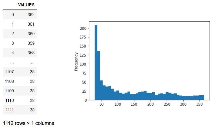
As we can see, the Values column does not resemble the Normal Distribution graph. It looks somewhat like an exponential distribution.

如我们所见，“值”列与正态分布图不同。 它看起来有点像指数分布。

Let’s pick samples from this distribution, calculate their means, and plot the sampling distribution.

让我们从该分布中选择样本，计算其均值，然后绘制采样分布图。

Now, the distribution graph for the samples looks like,

现在，样本的分布图如下所示：

Surprisingly, the Distribution of the sample_means we obtained from the Values Column, which is far from Normal Distribution, is still very much a Normal Distribution.

令人惊讶的是，我们从“值”列中获得的sample_means的分布与正态分布相去甚远，仍然非常接近正态分布。

Let’s compare the sample_means Mean value to its parent Mean value.

让我们将sample_means平均值与其父平均值进行比较。

sample_means.mean()
# The Output will be
130.39213999999996df1.Value.mean()
#The Output is
130.4181654676259

As we can see, the sample_means mean value and original dataset’s mean value are both similar.

如我们所见， sample_means平均值和原始数据集的平均值都相似。

Similarly, the standard deviation of sample mean is sample_means.std() =13.263962580003142

同样，样本均值的标准偏差为sample_means.std() = 13.263962580003142

That value should be quite close to df1.Value.std()/np.sqrt(samp_size) =14.060457446377631

该值应非常接近df1.Value.std()/np.sqrt(samp_size) = 14.060457446377631

Let’s compare the Distribution graphs of each Dataset with it’s corresponding sampling distribution.

让我们比较每个数据集的分布图及其对应的采样分布。

Image by Author

图片作者

As we can see, irrespective of the original dataset’s distribution, the sampling distribution resembles the Normal Distribution Curve.

如我们所见，无论原始数据集的分布如何，采样分布都类似于正态分布曲线。

There’s only one thing to consider now, i.e., Sample Size. We’ll observe that, as the sample size increases, the sampling distribution will approximate a normal distribution even more closely.

现在只有一件事要考虑，即样本数量。 我们将观察到，随着样本数量的增加，样本分布将更加接近正态分布。

样本量对抽样分布的影响 (Effect of Sample Size on the Sampling Distribution)

Let’s create different Sizes of samples and plot the corresponding distribution graphs.

让我们创建不同大小的样本并绘制相应的分布图。

Now, the Distribution Graph for Sample Sizes of 3, 10, 30, 50, 100, 200 looks like,

现在，样本量为3、10、30、50、100、200的分布图看起来像，

Distribution of Different Sample Sizes

不同样本量的分布

As we can observe, the distribution graph for Sample Size 3 & 10 does not resemble Normal Distribution. Still, from the Sample Size 30 as the Sample Size increases, the Sample Distribution resembles Normal Distribution.

如我们所见，样本大小3和10的分布图与正态分布不相似。 但是，随着样本数量的增加，样本数量从30开始，样本分布类似于正态分布。

As a rule of thumb, we can say that a sample size of 30 or above is ideal for concluding that the sampling distribution is nearly normal, and further inferences can be drawn from it.

根据经验，可以断定样本大小为30或更大，可以断定样本分布几乎是正态的，并且可以从中得出进一步的推论。

Through this Python Code, we can conclude that CLT’s following three properties hold.

通过此Python代码，我们可以得出结论CLT的以下三个属性成立。

1. Sampling Distribution Mean(μₓ¯) = Population Mean(μ)

   抽样分布平均值(μₓ) = 总体平均值(μ)

2. Sampling distribution’s standard deviation (Standard error) = σ/√n

   抽样分布的标准偏差( 标准误差 )= σ/√n

3. For n > 30, the sampling distribution becomes a normal distribution.

   当n> 30时 ，采样分布变为正态分布 。

使用CLT估计均值 (Estimating Mean Using CLT)

The mean commute time of 30000 employees (μ)= 36.6 (sample mean) + some margin of error. We can find this margin of error using the CLT (central limit theorem). Now that we know what the CLT is let’s see how we can find the error margin.

30000名员工的平均通勤时间(μ) = 36.6( 样本均值 )+一定的误差范围。 我们可以使用CLT(中心极限定理)找到这种误差范围。 现在我们知道了CLT是什么，让我们看看如何找到误差容限。

Let’s say we have the mean commute time of 100 employees is X¯=36.6 min, and the Standard Deviation of the sample is S=10 min. Using CLT, we can infer that,

假设我们有100名员工的平均通勤时间是X = 36.6分钟 ，样本的标准偏差是S = 10分钟 。 使用CLT，我们可以推断出

1. Sampling Distribution Mean(μₓ¯) = Population Mean(μ)
   抽样分布均值(μ)=总体均值(μ)
2. Sampling Distributions’ Standard Deviation = σ/√n ≈S/√n = 10/√100 = 1
   抽样分布的标准偏差=σ/√n≈S/√n= 10 /√100= 1

3. Since Sampling Distribution is a Normal Distribution

   由于采样分布是正态分布

   P(μ-2 < 36.6 < μ+2) = 95.4%, we get this value by 1–2–3 Rule of Normal Distribution Curve.

   P(μ-2<36.6 <μ+ 2)= 95.4％，我们通过正态分布曲线的1–2–3规则获得该值。

   P(μ-2 < 36.6 < μ+2) = P(36.6–2< μ < 36.6+2) = 95.4%

   P(μ-2<36.6 <μ+ 2)= P(36.6–2 <μ<36.6 + 2)= 95.4％

You can find the standard distribution curve, Z-Table, and its properties in my previous article, “Inferential Statistics.”

您可以在我之前的文章“ 推断统计量 ”中找到标准分布曲线，Z表及其属性。

Now, we can say that there is a 95.4% probability that the Population Mean(μ) lies between (36.6–2, 36.6+2). In other words, we are 95.4% confident that the error in estimating the mean ≤ 2.

现在，我们可以说，总体均值(μ)介于(36.6–2，36.6 + 2)之间的可能性为95.4％。 换句话说，我们有95.4％的信心认为平均值均值≤2的误差。

Hence the probability associated with the claim is called confidence level (Here it is 95.4%).The maximum error made in the sample mean is called the margin of error (Here it is 2min).The final interval of value is called confidence interval {Here it is: (34.6, 38.6)}

因此，与索赔相关的概率称为置信度 (此处为95.4％)。样本均值中的最大误差称为误差余量 (此处为2min)。最后的值间隔称为置信区间 {它是：(34.6，38.6)}

We can generalize this concept in the following manner.

我们可以通过以下方式来概括这个概念。

Let’s say that we have a sample with sample size n, mean X¯, and standard deviation S. Now, the y% confidence interval (i.e., the confidence interval corresponding to a y% confidence level) for μ would be given by the range:

假设我们有一个样本，样本量为n，均值X和标准差S。现在，μ的y％置信区间 (即，与ay％置信水平相对应的置信区间)将由以下范围给出：

Confidence interval = (X — (Z* S/√n), X + (Z* S/√n))

置信区间=(X-(Z * S /√n ) ，X +(Z * S /√n))

where Z* is the Z-score associated with a y% confidence level.

其中Z *是与ay％置信度相关的Z分数 。

Some commonly used Z* values are given below:

以下是一些常用的Z *值：

Z* Values Z *值

That is is how we calculate the margin of error and estimate the value of the mean of the whole population with the help of samples.

这就是我们计算误差幅度并借助样本估算整个总体平均值的值的方式。

结论 (Conclusion)

As we have seen, it is beneficial to find the mean and standard deviation for only a small representative sample. We may have to do this because of time and money constraints. Using CLT properties, we can find the Population Mean(μ), Standard Error(σ/√n), and, most importantly, Confidence interval(y%). CLT is beneficial in polling results reported on the news with confidence intervals, Insurance, Banking, etc. That is all about CLT and its properties and how it can be useful in Data Science.

正如我们已经看到的，只为一个小的代表性样本找到平均值和标准偏差是有益的。 由于时间和金钱的限制，我们可能必须这样做。 利用CLT属性，我们可以找到总体平均值(μ)，标准误差(σ/√n)，以及最重要的是置信区间(y％)。 CLT有助于以置信区间， 保险，银行业等方式 轮询新闻报道的结果 。这一切都与CLT及其属性以及它如何在数据科学中有用有关。

Thank you for reading and Happy Coding!!!

感谢您的阅读和快乐编码！！！

在这里查看我以前有关Python的文章 (Check out my previous articles about Python here)

• Inferential Statistics: Data Analysis

  推论统计：数据分析

• Exploratory Data Analysis(EDA): Python

  探索性数据分析(EDA)：Python

• Indexing in Pandas Dataframe using Python

  使用Python在Pandas Dataframe中建立索引

• Seaborn: Python

  Seaborn：Python

• Pandas: Python

  熊猫：Python

• Matplotlib: Python

  Matplotlib：Python

• NumPy: Python

  NumPy：Python

• Data Visualization and its Importance: Python

  数据可视化及其重要性：Python

• Time Complexity and Its Importance in Python

  时间复杂度及其在Python中的重要性

翻译自: https://towardsdatascience.com/central-limit-theorem-clt-data-science-19c442332a32

clt框架