matplotpy 线图_线图的样式转换

matplotpy 线图

Generating Images From Line Drawings With ML

使用ML从线图生成图像

Here, I’ll walk through a machine learning project a recently did in a tutorial-like manner. It is an approach to generating full images in an artistic style from line drawings.

在这里，我将逐步学习最近以类似教程的方式进行的机器学习项目。 这是一种从线条图生成艺术风格的完整图像的方法。

数据集 (Dataset)

I trained on 10% of the Imagenet dataset. This is a dataset commonly used for benchmarks in computer vision tasks. The Imagenet dataset is not openly available; it is restricted to those undergoing research which requires use of it to compute performance benchmarks for comparing with other approaches. Therefore, it is typically required that you submit a request form. But if you are just using it casually, it is available here. I just wouldn’t use this for beyond anything beyond personal projects. Note that the dataset is very large, which is why I only used 1/10th of it to train my model. It consists of 1000 classes, so I used 100 of these image classes for training.

我对Imagenet数据集的10％进行了培训 。 这是通常用于计算机视觉任务中基准测试的数据集。 Imagenet数据集不公开； 它仅限于进行研究的人员，这些人员需要使用它来计算性能基准以与其他方法进行比较。 因此，通常需要提交一份申请表。 但是，如果您只是随意使用它，可以在此处获得 。 我只是不会将其用于个人项目之外。 请注意，数据集非常大，这就是为什么我仅使用数据集的1/10训练模型的原因。 它由1000个班级组成，因此我将其中100个图像班级用于训练。

I used Imagenet for a different personal project a few weeks ago, so I already had the large collection of files in Google Drive. Unfortunately, however, it took approimately 20 hours to upload these 140,000 images or so to Google Drive. It is necessary to train the model on Google Colab’s online GPU, but this requires you upload the images to Google Drive, as you aren’t hosting your coding environment locally.

几周前，我将Imagenet用于另一个个人项目，因此我已经在Google云端硬盘中收集了大量文件。 不幸的是，将这140,000张图片上传到Google云端硬盘大约需要20个小时。 必须在Google Colab的在线GPU上训练模型，但这需要将图像上传到Google云端硬盘，因为您不在本地托管编码环境。

数据输入管道 (Data Input Pipeline)

I have a Colab Pro account, but even with the additional RAM, I certainly can’t handle 140,000 line drawing, each of 256x256 pixels in size, along with their 256x256 pixel colored counterparts. Hence, I have to load in the data on-the-go using a TensorFlow data input pipeline.

我有一个Colab Pro帐户，但是即使有额外的RAM，我当然也无法处理140,000线条图，每个线条图的大小为256x256像素，以及它们的256x256像素彩色对应线。 因此，我必须使用TensorFlow数据输入管道来不断加载数据。

Before we start to set up the pipeline, let’s import the required libraries (these are all of the import statements in my code):

在开始设置管道之前，让我们导入所需的库(这些是我代码中的所有import语句)：

import matplotlib.pyplot as plt
import numpy as np
import cv2
from tqdm.notebook import tqdm
import glob
import random
import threading, queuefrom tensorflow.keras.models import *
from tensorflow.keras.layers import *
from tensorflow.keras.optimizers import *
from tensorflow.keras.regularizers import *
from tensorflow.keras.utils import to_categorical
import tensorflow as tf

Now, let’s load the filepaths which refer to each image in our subset of Imagenet, assuming you have uploaded them to Drive under the appropriate directory structure and connection your Google Colab instance to your Google Drive.

现在，假设您已将它们上传到Imagenet子集中的每个图像，请假定它们已在适当的目录结构下上传到云端硬盘，并将您的Google Colab实例连接到您的Google Drive。

filepaths = glob.glob("drive/My Drive/1-100/**/*.JPEG")# Shuffle the filepaths
random.shuffle(filepaths)

If you don’t want to use the glob module, you can use functions from theos library, which are often more efficient.

如果您不想使用glob模块，则可以使用os库中的函数，这些函数通常效率更高。

Here’s a few helper functions I need:

这是我需要的一些辅助功能：

• Normalizing data
  规范化数据

• Posterizing image data

  海报图像数据

def normalize(x):
  return (x - x.min()) / (x.max() - x.min())

后发化 (Posterization)

The aforementioned process of posterization takes an image as input and transforms smooth gradients into more clearly-separated color sections by rounding color values to some nearest value. Here’s an example:

前述的后代化过程将图像作为输入，并且通过将颜色值四舍五入到某个最接近的值，将平滑的渐变转换为更清晰分离的颜色部分。 这是一个例子：

As you can see, the resulting image has less smooth gradients, which are replaced with separated color sections. The reason I am implementing this is because I can limit the output images to a set of colors, allowing me to format the learning problem as a classification problem across each pixel in an image. For each available color, I assign a label. The model outputs an image of shape (height, width, num_colors) activated by a softmax function over the last channel, num_colors. Given a variable num_values, I allow all combinations of RGB where the color values are limited to np.arange(0, 255, 255 / num_values). This means that num_colors = num_values ** 3. Here’s an example:

如您所见，生成的图像具有较少的平滑渐变，将其替换为单独的颜色部分。 之所以执行此操作，是因为我可以将输出图像限制为一组颜色，从而可以将学习问题格式化为图像中每个像素的分类问题。 对于每种可用颜色，我分配一个标签。 模型输出在最后一个通道num_colors上由softmax函数激活的形状(height, width, num_colors) num_colors 。 给定变量num_values ，我允许将RGB的所有组合(其中颜色值限制为np.arange(0, 255, 255 / num_values) 。 这意味着num_colors = num_values ** 3 。 这是一个例子：

Posterization

后发化

For an example of how I implemented this, here’s a demonstration:

有关如何实现此功能的示例，下面是一个演示：

def get_nearest_color(color, colors):
  """
  Args:
   - color: A vector of size 3 representing an RGB color
   - colors: NumPy array of shape (num_colors, 3)
  Returns:
   - The index of the color in the provided set of colors that is
     closest in value to the provided color
  """  return np.argmin([np.linalg.norm(color - c) for c in colors])def posterize_with_limited_colors(image, colors):
  """
  Args:
   - colors: NumPy array of shape (num_colors, 3)
  Returns:
   - Posterized image of shape (height, width, 1), where each value 
     is an integer label associated with a particular index of the
     provided colors array
  """  image = normalize(image)
  posterized = np.array([[get_nearest_color(x, colors) for x in y] for y in image])
  return posterized

边缘提取 (Edge Extraction)

In order to create the input data from our colored images, we need a method of extracting edges from an image which are akin to a trace or line drawing.

为了从我们的彩色图像创建输入数据，我们需要一种从图像中提取类似于轨迹或线条图的边缘的方法。

We’ll be using the Canny edge detection algorithm. Let’s write our helper function, which inputs the path to an image and output the associated example/(X, Y) training pair, comprised of a posterization of the colored input, alongside the black and white edge extraction:

我们将使用Canny边缘检测算法 。 让我们编写我们的辅助函数，该函数输入图像的路径并输出相关的example /(X，Y)训练对，该训练对由彩色输入的后代化以及黑色和白色边缘提取组成：

def preprocess(path):
  color = cv2.imread(path)
  color = cv2.resize(color, input_image_size)  # Assuming your pipelines generator function ignores None
  if color.shape < input_image_size:
    return None, None  color = (normalize(color) * 255).astype(np.uint8)  gray = cv2.cvtColor(color, cv2.COLOR_RGB2GRAY
  # Removes noise while preserving edges
  filtered = cv2.bilateralFilter(gray, 3, 60, 120)  # Automatically determine threshold for edge detection algorithm
  # based upon the median color value of the image
  m = np.median(filtered)
  preservation_factor = 0.33
  low = max(0, int(m - 255 * preservation_factor))
  high = int(min(255, m + 255 * preservation_factor))
  filtered_edges = cv2.Canny(filtered, low, high)
  filtered_edges = normalize(filtered_edges)
  filtered_edges = np.expand_dims(filtered_edges, axis = -1)  color = cv2.resize(color, output_image_size)
  color /= 255.
  color = posterize_with_limited_colors(color, colors)  return filtered_edges, color

The automatic Canny edge detection is just my modification to the small function used in this article.

自动Canny边缘检测只是我的变更而使用的小功能， 此文章。

管道 (The Pipeline)

As I said, I’m loading in data on-the-spot using an input pipeline. Therefore, I need to define a generator object to load in this data when needed. My generator function is simple because we basically just defined it. All it adds is filtering out the None outputs of the preprocess function (images of lower resolution than input_image_size and filtering out any results containing nan or inf values.

正如我所说，我正在使用输入管道现场加载数据。 因此，我需要定义一个生成器对象，以便在需要时加载此数据。 我的生成器函数很简单，因为我们基本上只是定义了它。 它添加的所有内容就是过滤掉preprocess功能的None输出(分辨率低于input_image_size图像，并过滤掉所有包含nan或inf值的结果。

def generate_data(paths):
  for path in paths:
    edges, color = preprocess(path.decode())
    if not edges is None:
      if not np.any(np.isnan(edges)) or np.any(np.isnan(color)):
        if not np.any(np.isinf(edges)) or np.any(np.isinf(color))):
          # Yield the clean data
          yield edges, color

I use (128, 128) for both input_image_size and output_image_size. A 128x128 pixel image isn’t that low-resolution, so there’s no significant disadvantage for our purposes. Also, Imagenet images are typically much higher resolution, so we can go higher if desired.

我将(128, 128)用作input_image_size和output_image_size 。 128x128像素的图像并不是那么低分辨率，因此对于我们的目的而言，没有明显的缺点。 同样，Imagenet图像通常具有更高的分辨率，因此如果需要，我们可以提高分辨率。

Now let’s build the pipeline. I’m using multithreading for improved speeds. TensorFlow’s.interleave()allows us to do this:

现在，我们来构建管道。 我正在使用多线程来提高速度。 TensorFlow的.interleave()允许我们执行以下操作：

thread_names = np.arange(0, 8).astype(str)
dataset = tf.data.Dataset.from_tensor_slices(thread_names)dataset = dataset.interleave(lambda x:
  tf.data.Dataset.from_generator(
    generate_data,
    output_types = (tf.float32, tf.float32),
    output_shapes = ((*input_image_size, 1),
                     (*output_image_size, 1)),
    args = (train_paths,)),
    cycle_length = 8,
    block_length = 8,
    num_parallel_calls = 8)dataset = dataset.batch(batch_size).repeat()

测试管道 (Testing The Pipeline)

Let’s load in a training example through our pipeline:

让我们通过管道加载一个培训示例：

One training example with input line drawing/edges (right) and output colorization (left)

一个带有输入线图/边线(右)和输出着色(左)的训练示例

It’s exactly as desired. Note that the image depicted on the left is not exactly what was outputted by the pipeline. Recall that the pipeline is returning the index referring to the color of each pixel. I simply referred to each associated color to create the visualization. Here’s an example of one that came out much simpler.

完全符合您的要求。 请注意，左侧描绘的图像与管道输出的图像不完全相同。 回想一下，管道正在返回引用每个像素颜色的索引。 我只是简单地引用了每种关联的颜色来创建可视化。 这是一个简单得多的例子。

Simpler training example

更简单的培训示例

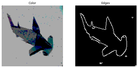
You’ll see that on the left we have the output, posterized color image, which partially resembles a painting. On the right, you see the input edge extraction, which resembles a sketch.

您会看到左侧有输出的，海报化的彩色图像，其部分类似于绘画。 在右侧，您会看到类似于草图的输入边缘提取。

Of course not all training examples will have as good of an edge extraction than others. When the colors are more difficult to separate, the resulting outline might be a little noisy and/or scattered. However, this was the most accurate method for extracting edges I could think of.

当然，并非所有的训练示例都具有比其他示例更好的边缘提取能力。 当颜色更难以分离时，结果轮廓可能会有点吵杂和/或分散。 但是，这是我想到的最精确的边缘提取方法。

模型架构 (Model Architecture)

Let’s move on to the model architecture.

让我们继续进行模型架构。

I begin at input_image_size = (128, 128), thus making the input of shape (128, 128, 1) after expanding the last axis. I decrease the layer input shape by a power of 2 until it equals 1. Then, I apply two more convolutional layers with stride = 1, because we can’t decrease the shape of the first two axes any further. Then, I perform the reverse with transposed layers. Each convolutional layer has padding = 'valid' and there is a batch normalization layer between each convolutional layer. All convolution layers have ReLU activation, except the last, which of course has softmax activation over the final one-hot-encoded color-label channel.

我从input_image_size = (128, 128) ，因此在扩展最后一个轴后进行形状输入input_image_size = (128, 128) (128, 128, 1) 。 我将层输入形状减小2的幂，直到等于1。然后，再应用两个卷积层，其stride = 1 ，因为我们不能再减小前两个轴的形状。 然后，我对转置图层执行相反的操作。 每个卷积层的padding = 'valid'并且每个卷积层之间都有一个批处理归一化层。 除最后一层外，所有卷积层均具有ReLU激活，最后一层当然在最终的一个热编码颜色标签通道上具有softmax激活。

_________________________________________________________________ Layer (type)                 Output Shape              Param #    ================================================================= input_35 (InputLayer)        [(None, 128, 128, 1)]     0          _________________________________________________________________ conv2d_464 (Conv2D)          (None, 64, 64, 3)         30         _________________________________________________________________ batch_normalization_388 (Bat (None, 64, 64, 3)         12         _________________________________________________________________ conv2d_465 (Conv2D)          (None, 32, 32, 9)         252        _________________________________________________________________ batch_normalization_389 (Bat (None, 32, 32, 9)         36         _________________________________________________________________ conv2d_466 (Conv2D)          (None, 16, 16, 27)        2214       _________________________________________________________________ batch_normalization_390 (Bat (None, 16, 16, 27)        108        _________________________________________________________________ conv2d_467 (Conv2D)          (None, 8, 8, 81)          19764      _________________________________________________________________ batch_normalization_391 (Bat (None, 8, 8, 81)          324        _________________________________________________________________ conv2d_468 (Conv2D)          (None, 4, 4, 243)         177390     _________________________________________________________________ batch_normalization_392 (Bat (None, 4, 4, 243)         972        _________________________________________________________________ conv2d_469 (Conv2D)          (None, 2, 2, 729)         1595052    _________________________________________________________________ batch_normalization_393 (Bat (None, 2, 2, 729)         2916       _________________________________________________________________ conv2d_470 (Conv2D)          (None, 1, 1, 2187)        14351094   _________________________________________________________________ batch_normalization_394 (Bat (None, 1, 1, 2187)        8748       _________________________________________________________________ conv2d_471 (Conv2D)          (None, 1, 1, 2187)        43048908   _________________________________________________________________ batch_normalization_395 (Bat (None, 1, 1, 2187)        8748       _________________________________________________________________ conv2d_472 (Conv2D)          (None, 1, 1, 2187)        43048908   _________________________________________________________________ batch_normalization_396 (Bat (None, 1, 1, 2187)        8748       _________________________________________________________________ conv2d_transpose_229 (Conv2D (None, 1, 1, 2187)        43048908   _________________________________________________________________ batch_normalization_397 (Bat (None, 1, 1, 2187)        8748       _________________________________________________________________ conv2d_transpose_230 (Conv2D (None, 1, 1, 2187)        43048908   _________________________________________________________________ batch_normalization_398 (Bat (None, 1, 1, 2187)        8748       _________________________________________________________________ conv2d_transpose_231 (Conv2D (None, 2, 2, 2187)        43048908   _________________________________________________________________ batch_normalization_399 (Bat (None, 2, 2, 2187)        8748       _________________________________________________________________ conv2d_transpose_232 (Conv2D (None, 4, 4, 2187)        43048908   _________________________________________________________________ batch_normalization_400 (Bat (None, 4, 4, 2187)        8748       _________________________________________________________________ conv2d_transpose_233 (Conv2D (None, 8, 8, 729)         14349636   _________________________________________________________________ batch_normalization_401 (Bat (None, 8, 8, 729)         2916       _________________________________________________________________ conv2d_transpose_234 (Conv2D (None, 16, 16, 243)       1594566    _________________________________________________________________ batch_normalization_402 (Bat (None, 16, 16, 243)       972        _________________________________________________________________ conv2d_transpose_235 (Conv2D (None, 32, 32, 81)        177228     _________________________________________________________________ batch_normalization_403 (Bat (None, 32, 32, 81)        324        _________________________________________________________________ conv2d_transpose_236 (Conv2D (None, 64, 64, 27)        19710      _________________________________________________________________ up_sampling2d_1 (UpSampling2 (None, 128, 128, 27)      0          _________________________________________________________________ batch_normalization_404 (Bat (None, 128, 128, 27)      108        ================================================================= Total params: 290,650,308 Trainable params: 290,615,346 Non-trainable params: 34,962 _________________________________________________________________

训练 (Training)

Let’s create some lists to store out metrics throughout training.

让我们创建一些列表以存储整个培训中的指标。

train_losses, train_accs = [], []

Also, a variable for the number of training epochs

另外，一个训练时期数的变量

epochs = 100

And here’s our training script

这是我们的训练脚本

for epoch in range(epochs):
  random.shuffle(filepaths)
  history = model.fit(dataset,
                      steps_per_epoch = steps_per_epoch,
                      use_multiprocessing = True,
                      workers = 8,
                      max_queue_size = 10)  train_loss = np.mean(history.history["loss"])
  train_acc = np.mean(history.history["accuracy"])  train_losses = train_losses + history.history["loss"]
  train_accs = train_accs + history.history["accuracy"]  print ("Epoch: {}/{}, Train Loss: {:.6f}, Train Accuracy: {:.6f}, Val Loss: {:.6f}, Val Accuracy: {:.6f}".format(epoch + 1, epochs, train_loss, train_acc, val_loss, val_acc))  if epoch > 0:
    fig = plt.figure(figsize = (10, 5))
    plt.subplot(1, 2, 1)
    plt.plot(train_losses)
    plt.xlim(0, len(train_losses) - 1)
    plt.xlabel("Epoch")
    plt.ylabel("Loss")
    plt.title("Loss")
    plt.subplot(1, 2, 2)
    plt.plot(train_accs)
    plt.xlim(0, len(train_accs) - 1)
    plt.ylim(0, 1)
    plt.xlabel("Epoch")
    plt.ylabel("Accuracy")
    plt.title("Accuracy")
    plt.show()  model.save("model_{}.h5".format(epoch))
  np.save("train_losses.npy", train_losses)
  np.save("train_accs.npy", train_accs)

工作正在进行中… (Work In Progress…)

This is my second day working on this project; it’s currently in the works, so I don’t have a definitive model architecture yet. Hence, the model presented in the last section is likely not finalized. By tomorrow, I’ll update this post with results, a GitHub link to my code, and the final model architecture I settled on.

这是我第二天在做这个项目。 它目前正在开发中，所以我还没有确定的模型架构。 因此，最后一节中介绍的模型可能无法最终确定。 到明天，我将用结果，代码的GitHub链接以及确定的最终模型体系结构更新此帖子。

翻译自: https://medium.com/@ryanrudes/style-transfer-for-line-drawings-3c994492b609

matplotpy 线图