总体方差的充分统计量_R方是否衡量预测能力或统计充分性？

总体方差的充分统计量

The way that R-squared shouldn’t be utilized for choosing if you have a satisfactory model is illogical and is once in a while clarified unmistakably. This exhibit diagrams how R-squared integrity of-fit functions in relapse investigation and relationships while demonstrating why it’s anything but a proportion of measurable sufficiency, so ought not to propose anything about future prescient execution.

如果您有满意的模型，不应该使用R平方的方法进行选择是不合逻辑的，而且有时会明确地加以阐明。 该图说明了在复发调查和关系中拟合函数的R平方完整性如何进行，同时说明了为什么它只是可测量的充足程度的一部分，因此不应提出任何关于未来先行执行的建议。

The R-squared Goodness-of-Fit measure is one of the most broadly accessible insights going with the yield of relapse investigation in factual programming. Maybe incompletely because of its far-reaching accessibility, it is additionally one of the frequently misjudged ones.

R平方拟合优度度量是事实编程中复发调查的结果之一，是使用最广泛的见解之一。 由于它的深远的可访问性，它可能是不完整的，它也是经常被误判的一种。

Initial, a concise update on R-squared (R2). In a relapse with a solitary free factor, R2 is determined as the proportion between the variety clarified by the model and the all-out watched variety. It is regularly called the coefficient of assurance and can be deciphered as the extent of variety clarified by the presented indicator. In such a case, it is proportionate to the square of the convection coefficient of the watched and fitted estimations of the variable. In various relapse, it is known as the coefficient of different assurance and is regularly determined utilizing a modification that punishes it is worth relying upon the number of indicators utilized.

最初，是对R平方(R2)的简要更新。 在具有单独的自由因子的复发中，R2被确定为模型阐明的品种与全面观察的品种之间的比例。 通常将其称为保证系数，并且可以根据所提供的指标所阐明的多样性程度来进行解密。 在这种情况下，它与变量的监视和拟合估计的对流系数的平方成比例。 在各种复发中，它被称为不同保证系数，并定期根据惩罚的修改来确定，这值得依赖所使用的指标数量。

In neither of these cases, be that as it may, does R2 measure whether the correct model was picked, and therefore, it doesn’t quantify the prescient limit of the acquired fit. This is accurately noted in numerous sources, yet not many clarify that factual sufficiency is essential for effectively deciphering a coefficient of assurance. Special cases incorporate Spanos 2019 [1] wherein one can peruse “underscore that the above measurements [R-squared and others] are significant just for the situation where the evaluated straight relapse model is factually sufficient,” and Hagquist and Stenbeck (1998).[2] It is much rarer to see instances of why that is the situation with an exemption being Ford 2015.[3]

在这两种情况下，R2都不会测量是否选择了正确的模型，因此，它不会量化获得的拟合的先验极限。 许多来源都准确地指出了这一点，但很少有人澄清事实的充分性对于有效地破译保证系数至关重要。 特殊情况包括Spanos 2019 [1]，其中人们可以细读“强调以上测量值(R平方和其他测量值)仅对于所评估的直接复发模型实际上足够的情况才有意义”，以及Hagquist和Stenbeck(1998年)。 [2] 很少见到为什么会有这种情况的情况被豁免为福特2015。[3]

The current article incorporates a more extensive arrangement of models that explain the job and constraints of the coefficient of assurance. To keep it reasonable, just a single variable relapse is analyzed. The Appeal of R-squared

当前文章包含了更广泛的模型排列，这些模型解释了保证系数的工作和约束。 为了使其合理，仅分析单个变量复发。 R平方的诉求

First, let us examine the utility of R2 and to see why it is so easy to incorrectly interpret it as a measure of statistical adequacy and predictive accuracy when it is neither. Using a comparison with the simple linear correlation coefficient will help us understand why it behaves the way it does.

首先，让我们检查一下R2的效用，看看为什么容易错误地将其解释为统计上的充分性和预测准确性的度量，而两者都不是。 与简单的线性相关系数进行比较将有助于我们理解其行为方式。

Figure 1 below is based on extracted data from 32 price offers for second-hand cars of one high-end model. The idea is to examine the relationship between car age (x-axis) and price (y-axis, in my local currency unit).

下面的图1基于从一种高端模型的二手车的32种价格报价中提取的数据。 这个想法是要检查车龄(x轴)和价格(y轴，以我的本地货币单位)之间的关系。

Entering the information into a connection coefficient adding machine, we acquire a Pearson’s r of — 0.8978 (p-esteem 0 to the eighth decimal spot, 95%CI: — 0.9493, — 0.7992). These outcomes in an agreeable R2 of 0.8059, which would, truth be told, be viewed as high by numerous guidelines. The connection figuring is comparable to running a straight relapse. Eyeballing the fit makes it clear that it can probably be improved by picking a non-straight relationship from the exponential family all things considered:

将信息输入到连接系数加法器中，我们获得的皮尔逊r为-0.8978(p估计0到第八个小数点，95％CI：-0.9493，-0.7992)。 这些结果的可接受的R2为0.8059，事实证明，许多指导方针都认为这是很高的。 连接方式可与连续重复进行比较。 眼神看似合体，很明显，可以通过从指数家族中选择所有考虑的非直线关系来改善这种关系：

Figure 2

图2

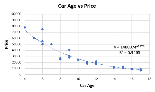
The fit acquired with the relapse condition that appeared in Figure 2 above has an R2 estimation of 0.9465, this one is constrained to supplant the straight with the exponential model. As the exponential model clarifies a greater amount of the difference, one may think it is a superior portrayal of the hidden information creating an instrument, and maybe this likewise implies it will have better prescient exactness. That is the natural intrigue of utilizing R-squared to pick between one model and another. Notwithstanding, this isn’t really so as the following parts will illustrate.

在上面的图2中出现的复发情况下获得的拟合的R2估计值为0.9465，这被约束为用指数模型代替直线。 随着指数模型澄清了更大的差异，人们可能会认为这是对创建工具的隐藏信息的更好描述，也许这也暗示着它将具有更好的先验准确性。 利用R平方在一个模型和另一个模型之间进行选择是很自然的事情。 尽管如此，以下部分将对此进行说明。

不同的底层模型，相同的R平方？ (Different Underlying Model, Same R-squared?)

Imagine a scenario in which disclosed to you that you can get the equivalent R2 measurement for a direct relapse of two particular datasets while realizing that the fundamental model is very extraordinary in each set. This can be shown by a straightforward reenactment. The accompanying R code produces indicator and reaction esteems dependent on two separate genuine models — one is direct, and the other is exponential:

想象一下一个场景，在该场景中向您披露，您可以在两个特定数据集直接重复使用的同时获得等效的R2度量，同时意识到基本模型在每个集合中都非常出色。 这可以通过简单的重新制定来体现。 随附的R代码根据两个独立的真实模型来产生指标和React评价-一个是直接的，另一个是指数的：

set.seed(1);                           # set seed for replicability
x <- seq(1,10,length.out = 1000)       # predictor values
y <- 1 + 1.5*x + rnorm(1000, 0, 0.80)  # response values produced as a linear function of x and random noise with sd of 0.649
summary(lm(y ~ x))$r.squared           # print R-squared for the linear model
y <- x^2 + rnorm(1000, 0, 0.80)        # response values produced as an exponential function of x and random noise with sd of 1.377
summary(lm(y ~ x))$r.squared           # print R-squared for the exponential model

The consequence of the straight model fit is R2 = 0.957 for both. In any case, we realize that one lot of information originates from a direct reliance and another from an exponential one. This can be additionally investigated utilizing the plots of the reaction variable y, as appeared in Figure 3.

两者的直线模型拟合结果均为R2 = 0.957。 无论如何，我们意识到，大量信息来自直接依赖，而另一半则来自指数依赖。 可以使用React变量y的图对此进行额外研究，如图3所示。

Figure 3

图3

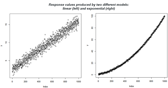
On the off chance that one uses an R-squared edge to acknowledge a model, they would probably acknowledge a straight model for the two conditions. In spite of a similar R-squared measurement created, the prescient legitimacy would be somewhat extraordinary relying upon what the genuine reliance is. In the event that it is really direct, at that point the prescient exactness would be very acceptable. Else, it will be a lot more unfortunate. In this sense, R-Squared is certainly not a decent proportion of prescient mistake. The standard blunder would have been a vastly improved guide being about multiple times littler in the principal case.

在使用R平方边确认模型的机会很小的情况下，他们可能会在两种情况下都承认一个直线模型。 尽管创建了类似的R平方测量值，但根据真正依赖程度的不同，预先确定的合法性还是有些不同。 如果确实是直接的，那么在那一点上预先确定的准确性是可以接受的。 否则，将会更加不幸。 从这个意义上说，R-Squared当然不是先天错误的一部分。 标准错误将是一个大大改进的指南，在主要情况下要少很多倍。

低R平方不一定表示统计模型不足 (Low R-squared Doesn’t Necessarily Mean an Inadequate Statistical Model)

In the principal model, the standard deviation of the irregular commotion was kept the equivalent, and we changed just the kind of reliance. In any case, the coefficient of assurance is fundamentally impacted by the scattering of the arbitrary mistake term, and this is the thing that we will look at straightaway. The code beneath produces mimicked R2 values for various degrees of the standard deviation of the blunder term for y while keeping the kind of reliance the equivalent. The information is produced with a satisfactory model for the blunder term, and the relationship is straight. It fulfills the straightforward relapse model on all records: ordinariness, zero mean, homoskedasticity, no autocorrelation, and no collinearity as only a solitary variable is included.

在主模型中，不规则运动的标准偏差保持相等，而我们仅更改了依赖类型。 无论如何，保证系数从根本上受到任意错误项的分散的影响，这就是我们将要看的东西。 下面的代码针对y的失误项的标准偏差的不同程度生成模仿的R2值，同时保持对等的依赖。 对于失误项，将使用令人满意的模型来生成信息，并且该关系是直接的。 它满足所有记录上简单明了的复发模型：通常，零均值，同方差，无自相关和共线性，因为仅包含一个单独变量。

r2 <- function(sd){
  x <- seq(1,10,length.out = 1000)       # predictor values
  y <- 2 + 1.2*x + rnorm(1000,0,sd = sd) # response values produced as a linear function of x and random noise with sd of sd
  summary(lm(y ~ x))$r.squared           # print R-squared
}sds <- seq(0.5,40,length.out = 40)       # generate sd values with a step of 0.5
res <- sapply(sds, r2)                   # calculate the function with each sd value
plot(res ~ sds, type="b", main="R-squared for different values of Sigma", xlab="Sigma (Standard Deviation)", ylab="Average R-squared")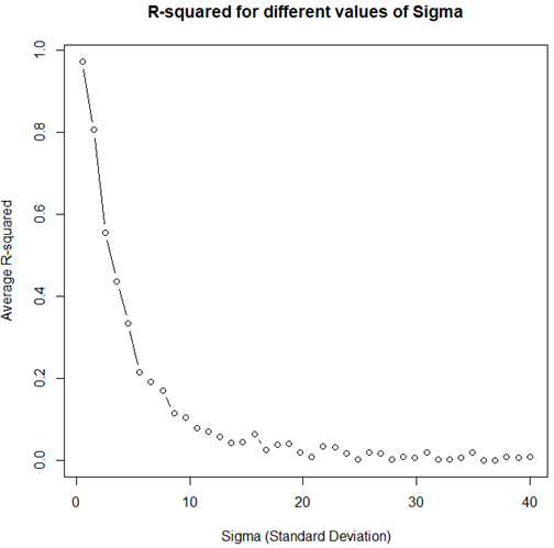

Figure 4

图4

Despite the fact that the measurable model fulfills all prerequisites and is in this manner very much indicated, with expanding change in the blunder term, the R2 esteem will in general zero. The above is an exhibit of why it can’t be utilized as a proportion of measurable insufficiency.

尽管可测量模型满足了所有先决条件，并且以这种方式非常明显地指出了这一点，但随着失误项的变化不断扩大，R2自尊通常将为零。 以上是为什么不能将其作为可衡量的供血不足比例使用的一种证明。

高R平方不一定表示适当的统计模型 (High R-squared Doesn’t Necessarily Mean an Adequate Statistical Model)

Something contrary to the above situation can occur if the model is miss-indicated at this point the standard deviation is adequately little. This will in general produce high R2 values as shown by running the code beneath.

如果模型在这一点上未正确指示，则标准偏差足够小，则可能会发生与上述情况相反的情况。 如下面的代码所示，这通常会产生较高的R2值。

r2 <- function(sd){
  x <- seq(1,10,length.out = 1000)       # predictor values
  y <- x^2 + rnorm(1000,0,sd = sd)       # response values produced as a linear function of x and random noise with sd of sd
  summary(lm(y ~ x))$r.squared           # print R-squared
}sds <- seq(0.5,40,length.out = 40)       # genearte sd values with a step of 0.5
res <- sapply(sds, r2)                   # calculate the function with each sd value
plot(res ~ sds, type="b", main="R-squared for different values of Sigma", xlab="Sigma (Standard Deviation)", ylab="Average R-squared")

It should produce a plot like the one shown in Figure 5.

它应该产生类似于图5所示的图。

Figure 5

图5

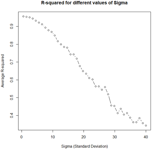
As clear, even with an unequivocally non-straight basic model, high R-squared qualities can be watched for a wide scope of sigma esteems. This implies even self-assertively high estimations of the measurement can’t really be taken as proof for model ampleness.

很明显，即使使用了明确的非直线型基本模型，对于广泛的sigma估计，也可以观察到高R平方质量。 这意味着，即使是对测量值的高估，也不能真正用作模型充裕度的证明。

结论 (conclusion)

Ideally, the above models fill in as an adequate outline of the threats of over-deciphering the coefficient of assurance. While it is a proportion of decency of-fit, it possibly increases meaning if the model is satisfactory as for the fundamental instrument producing the information. Utilizing it as a proportion of model ampleness isn’t justified, and to the degree to which homing in on the right model effects or prescient mistake, it’s anything but a proportion of it either. Regardless of whether that leaves any valuable spot for it at all is as yet a matter of discussion.

理想情况下，以上模型可作为过度解密保证系数威胁的适当概述。 虽然它是拟合优度的一部分，但对于产生信息的基本工具而言，如果模型令人满意，则可能会增加含义。 将其作为一定比例的模型充裕度是没有道理的，在某种程度上，归因于正确的模型效果或先天性的错误，也只是比例的一部分而已。 不管这是否给它留下任何有价值的地方，都仍在讨论中。

[1] Spanos A. (2019). “Probability Theory and Statistical Inference: Empirical Modeling with Observational Data.” Cambridge University Press. p.635

[1] Spanos A.(2019年)。 “概率论与统计推论：带有观测数据的经验建模。” 剑桥大学出版社 。 第635章

[2] Hagquist, C., Stenbeck, M. (1998) “Goodness of Fit in Regression Analysis — R 2 and G 2 Reconsidered.” Quality and Quantity. 32, pp.229–245

[2] Hagquist，C.，Stenbeck，M.(1998)“回归分析的拟合优度-重新考虑R 2和G 2。” 质量和数量。 32，第229–245页

[3] Ford C. (2015). “Is R-squared Useless?” https://data.library.virginia.edu/is-r-squared-useless/

[3]福特C.(2015)。 “ R平方没用吗？” https://data.library.virginia.edu/is-r-squared-useless/

Bio: Arpit Bhushan Sharma (B.Tech, 2016–2020) Electrical & Electronics Engineering, KIET Group of Institutions Ghaziabad, Uttar Pradesh, India. | Project Manager — Project4jungle | Chief Organising Officer — Waco | Project Manager— Edusmith | Student Member R10 IEEE | Student Member PES | Voice: +91 8445726929 | E-mail: bhushansharmaarpit@gmail.com

简介： Arpit布尚·夏尔马 ( B.Tech ，2016-2020)电气与电子工程学院，机构加济阿巴德的KIET集团，印度北方邦。 | 项目经理— Project4jungle | 韦科首席组织官| 项目经理— Edusmith | 学生会员R10 IEEE | 学生会员PES | 语音：+91 8445726929 | 电子邮件：bhushansharmaarpit@gmail.com

翻译自: https://medium.com/@bhushansharmaarpit/does-r-square-measure-the-predictive-capacity-or-statistical-sufficiency-73812bb95c38

总体方差的充分统计量