matlab中frequency,Scale to frequency

This example shows how the pseudo-frequency changes as you double the scale.

Construct a vector of scales with 10 voices per octave over five octaves.

vpo = 10;

no = 5;

a0 = 2^(1/vpo);

ind = 0:vpo*no;

sc = a0.^ind;

Verify that the range of scales covers five octaves.

log2(max(sc)/min(sc))

ans = 5.0000

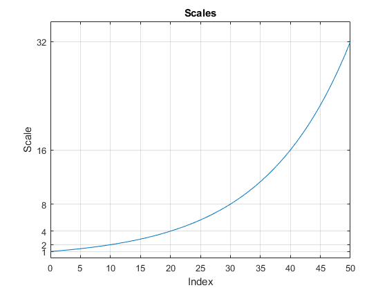
If you plot the scales, you can use a data cursor to confirm that the scale at index n+10 is twice the scale at index n. Set the y-ticks to mark each octave.

plot(ind,sc)

title('Scales')

xlabel('Index')

ylabel('Scale')

grid on

set(gca,'YTick',2.^(0:5))

Convert the scales to pseudo-frequencies for the real-valued Morlet wavelet. First, assume the sampling period is 1.

pf = scal2frq(sc,"morl");

T = [sc(:) pf(:)];

T = array2table(T,'VariableNames',{'Scale','Pseudo-Frequency'});

disp(T)

Scale Pseudo-Frequency

______ ________________

1 0.8125

1.0718 0.75809

1.1487 0.70732

1.2311 0.65996

1.3195 0.61576

1.4142 0.57452

1.5157 0.53605

1.6245 0.50015

1.7411 0.46666

1.8661 0.43541

2 0.40625

2.1435 0.37904

2.2974 0.35366

2.4623 0.32998

2.639 0.30788

2.8284 0.28726

3.0314 0.26803

3.249 0.25008

3.4822 0.23333

3.7321 0.2177

4 0.20313

4.2871 0.18952

4.5948 0.17683

4.9246 0.16499

5.278 0.15394

5.6569 0.14363

6.0629 0.13401

6.498 0.12504

6.9644 0.11666

7.4643 0.10885

8 0.10156

8.5742 0.094761

9.1896 0.088415

9.8492 0.082494

10.556 0.07697

11.314 0.071816

12.126 0.067006

12.996 0.062519

13.929 0.058332

14.929 0.054426

16 0.050781

17.148 0.047381

18.379 0.044208

19.698 0.041247

21.112 0.038485

22.627 0.035908

24.251 0.033503

25.992 0.03126

27.858 0.029166

29.857 0.027213

32 0.025391

Assume that data is sampled at 100 Hz. Construct a table with the scales, the corresponding pseudo-frequencies, and periods. Since there are 10 voices per octave, display every tenth row in the table. Observe that for each doubling of the scale, the pseudo-frequency is cut in half.

Fs = 100;

DT = 1/Fs;

pf = scal2frq(sc,"morl",DT);

T = [sc(:)/Fs pf(:) 1./pf(:)];

T = array2table(T,'VariableNames',{'Scale','Pseudo-Frequency','Period'});

T(1:vpo:end,:)

ans=6×3 table

Scale Pseudo-Frequency Period

_____ ________________ ________

0.01 81.25 0.012308

0.02 40.625 0.024615

0.04 20.313 0.049231

0.08 10.156 0.098462

0.16 5.0781 0.19692

0.32 2.5391 0.39385

Note the presence of the Δt=1Fs factor in scal2frq. This is necessary in order to achieve the proper scale-to-frequency conversion. The Δt is needed to adjust the raw scales properly. For example, with:

f = scal2frq(1,'morl',0.01);

You are really asking what happens to the center frequency of the mother Morlet wavelet, if you dilate the wavelet by 0.01. In other words, what is the effect on the center frequency if instead of ψ(t), you look at ψ(t/0.01). The Δt provides the correct adjustment factor on the scales.

You could have obtained the same results by first converting the scales to their adjusted sizes and then using scal2frq without specifyingΔt.

scadjusted = sc.*0.01;

pf2 = scal2frq(scadjusted,'morl');

max(pf-pf2)

ans = 0