


一. 算法概述
本文提出的SSD算法是一种直接预测目标类别和bounding box的多目标检测算法。与faster rcnn相比,该算法没有生成 proposal 的过程,这就极大提高了检测速度。针对不同大小的目标检测,传统的做法是先将图像转换成不同大小(图像金字塔),然后分别检测,最后将结果综合起来(NMS)。而SSD算法则利用不同卷积层的 feature map 进行综合也能达到同样的效果。文章的核心之一是同时采用lower和upper的feature map做检测。
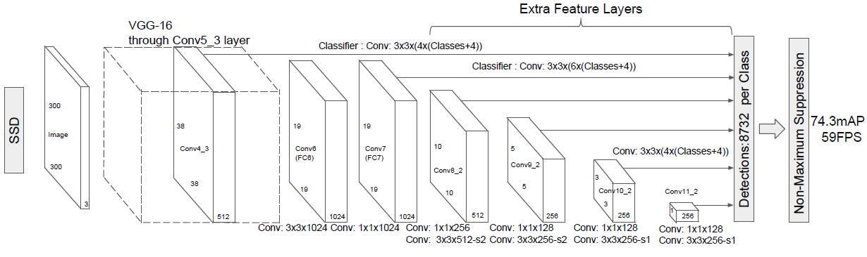
Fig.1 SSD 框架
算法的主网络结构是VGG16,将最后两个全连接层改成卷积层,并随后增加了4个卷积层来构造网络结构。对其中5种不同的卷积层的输出(feature map)分别用两个不同的 3×3 的卷积核进行卷积,一个输出分类用的confidence,每个default box 生成21个类别confidence;一个输出回归用的 localization,每个 default box 生成4个坐标值(x, y, w, h)。此外,这5个feature map还经过 PriorBox 层生成 prior box(生成的是坐标)。上述5个feature map中每一层的default box的数量是给定的(8732个)。最后将前面三个计算结果分别合并然后传给loss层。
二. Default box
文章的核心之一是作者同时采用lower和upper的feature map做检测。如图Fig 1 所示,这里假定有8×8和4×4两种不同的feature map。第一个概念是feature map cell,feature map cell 是指feature map中每一个小格子,如图中分别有64和16个cell。另外有一个概念:default box,是指在feature map的每个小格(cell)上都有一系列固定大小的box,如下图有4个(下图中的虚线框,仔细看格子的中间有比格子还小的一个box)。假设每个feature map cell有k个default box,那么对于每个default box都需要预测c个类别score和4个offset,那么如果一个feature map的大小是m×n,也就是有m*n个feature map cell,那么这个feature map就一共有(c+4)*k * m*n 个输出。这些输出个数的含义是:采用3×3的卷积核对该层的feature map卷积时卷积核的个数,包含两部分(实际code是分别用不同数量的3*3卷积核对该层feature map进行卷积):数量c*k*m*n是confidence输出,表示每个default box的confidence,也就是类别的概率;数量4*k*m*n是localization输出,表示每个default box回归后的坐标)。训练中还有一个东西:prior box,是指实际中选择的default box(每一个feature map cell 不是k个default box都取)。也就是说default box是一种概念,prior box是实际的选取。训练中一张完整的图片送进网络获得各个feature map,对于正样本训练来说,需要先将prior box与ground truth box做匹配,匹配成功说明这个prior box所包含的是个目标,但离完整目标的ground truth box还有段距离,训练的目的是保证default box的分类confidence的同时将prior box尽可能回归到ground truth box。 举个列子:假设一个训练样本中有2个ground truth box,所有的feature map中获取的prior box一共有8732个。那个可能分别有10、20个prior box能分别与这2个ground truth box匹配上。训练的损失包含定位损失和回归损失两部分。
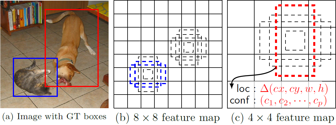
Fig.2 default boxes
作者的实验表明default box的shape数量越多,效果越好。
这里用到的 default box 和Faster RCNN中的 anchor 很像,在Faster RCNN中 anchor 只用在最后一个卷积层,但是在本文中,default box 是应用在多个不同层的feature map上。
那么default box的scale(大小)和aspect ratio(横纵比)要怎么定呢?假设我们用m个feature maps做预测,那么对于每个featuer map而言其default box的scale是按以下公式计算的:
$\vee$
$S_k=S_{min} + \frac{S_{max} - S_{min}}{m-1}(k-1), k\in{[1, m]}$
这里smin是0.2,表示最底层的scale是0.2;smax是0.9,表示最高层的scale是0.9。
至于aspect ratio,用$a_r$表示为下式:注意这里一共有5种aspect ratio
$a_r = \{1, 2, 3, 1/2, 1/3\}$
因此每个default box的宽的计算公式为:
$w_k^a=s_k\sqrt{a_r}$
高的计算公式为:(很容易理解宽和高的乘积是scale的平方)
$h_k^a=s_k/\sqrt{a_r}$
另外当aspect ratio为1时,作者还增加一种scale的default box:
$s_k^{'}=\sqrt{s_{k}s_{k+1}}$
因此,对于每个feature map cell而言,一共有6种default box。
可以看出这种default box在不同的feature层有不同的scale,在同一个feature层又有不同的aspect ratio,因此基本上可以覆盖输入图像中的各种形状和大小的object!
(训练自己的样本的时候可以在FindMatch()之后检查是否覆盖了所有得 ground truth box)
具体到代码 ssd_pascal.py 中是这样设计的:这里与论文中的公式有细微变化,自己体会。。。
mbox_source_layers = ['conv4_3', 'fc7', 'conv6_2', 'conv7_2', 'conv8_2', 'conv9_2']
# in percent %
min_ratio = 20
max_ratio = 90
step = int(math.floor((max_ratio - min_ratio) / (len(mbox_source_layers) - 2)))
min_sizes = []
max_sizes = []
for ratio in xrange(min_ratio, max_ratio + 1, step):
  min_sizes.append(min_dim * ratio / 100.)
  max_sizes.append(min_dim * (ratio + step) / 100.)
min_sizes = [min_dim * 10 / 100.] + min_sizes
max_sizes = [min_dim * 20 / 100.] + max_sizes
steps = [8, 16, 32, 64, 100, 300]
aspect_ratios = [[2], [2, 3], [2, 3], [2, 3], [2], [2]]
caffe 源码 prior_box_layer.cpp 中是这样提取 prior box 的:


 for (int h = 0; h < layer_height; ++h) {
    for (int w = 0; w < layer_width; ++w) {
      float center_x = (w + offset_) * step_w;
      float center_y = (h + offset_) * step_h;
      float box_width, box_height;
      for (int s = 0; s < min_sizes_.size(); ++s) {
        int min_size_ = min_sizes_[s];
        // first prior: aspect_ratio = 1, size = min_size
        box_width = box_height = min_size_;
        // xmin
        top_data[idx++] = (center_x - box_width / 2.) / img_width;
        // ymin
        top_data[idx++] = (center_y - box_height / 2.) / img_height;
        // xmax
        top_data[idx++] = (center_x + box_width / 2.) / img_width;
        // ymax
        top_data[idx++] = (center_y + box_height / 2.) / img_height;

        if (max_sizes_.size() > 0) {
          CHECK_EQ(min_sizes_.size(), max_sizes_.size());
          int max_size_ = max_sizes_[s];
          // second prior: aspect_ratio = 1, size = sqrt(min_size * max_size)
          box_width = box_height = sqrt(min_size_ * max_size_);
          // xmin
          top_data[idx++] = (center_x - box_width / 2.) / img_width;
          // ymin
          top_data[idx++] = (center_y - box_height / 2.) / img_height;
          // xmax
          top_data[idx++] = (center_x + box_width / 2.) / img_width;
          // ymax
          top_data[idx++] = (center_y + box_height / 2.) / img_height;
        }

        // rest of priors
        for (int r = 0; r < aspect_ratios_.size(); ++r) {
          float ar = aspect_ratios_[r];
          if (fabs(ar - 1.) < 1e-6) {
            continue;
          }
          box_width = min_size_ * sqrt(ar);
          box_height = min_size_ / sqrt(ar);
          // xmin
          top_data[idx++] = (center_x - box_width / 2.) / img_width;
          // ymin
          top_data[idx++] = (center_y - box_height / 2.) / img_height;
          // xmax
          top_data[idx++] = (center_x + box_width / 2.) / img_width;
          // ymax
          top_data[idx++] = (center_y + box_height / 2.) / img_height;
        }
      }
    }
  }
具体到每一个feature map上获得prior box时,会从这6种中进行选择。如下表和图所示最后会得到(38*38*4 + 19*19*6 + 10*10*6 + 5*5*6 + 3*3*4 + 1*1*4)= 8732个prior box。
| feature map | feature map size | min_size($s_k$) | max_size($s_{k+1}$) | aspect_ratio | step | offset | variance |
| conv4_3 | 38×38 | 30 | 60 | 1,2 | 8 | 0.50 | 0.1, 0.1, 0.2, 0.2 |
| fc6 | 19×19 | 60 | 111 | 1,2,3 | 16 | ||
| conv6_2 | 10×10 | 111 | 162 | 1,2,3 | 32 | ||
| conv7_2 | 5×5 | 162 | 213 | 1,2,3 | 64 | ||
| conv8_2 | 3×3 | 213 | 264 | 1,2 | 100 | ||
| conv9_2 | 1×1 | 264 | 315 | 1,2 | 300 |
三. 正负样本
将prior box 和 grount truth box 按照IOU(JaccardOverlap)进行匹配,匹配成功则这个prior box就是positive example(正样本),如果匹配不上,就是negative example(负样本),显然这样产生的负样本的数量要远远多于正样本。这里将前向loss进行排序,选择最高的num_sel个prior box序号集合 $D$。那么如果Match成功后的正样本序号集合$P$。那么最后正样本集为 $P - D\cap{P}$,负样本集为 $D - D\cap{P}$,这里利用num_sel控制最后正、负样本的比例在 1:3 左右。
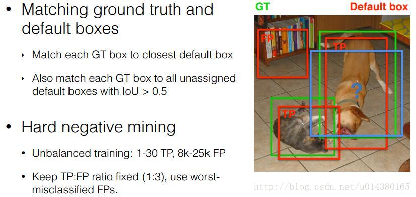
Fig.3 positive and negtive sample VS ground_truth box
1.正样本获得
我们已经在图上画出了prior box,同时也有了ground truth,那么下一步就是将prior box匹配到ground truth上,这是在 src/caffe/utlis/bbox_util.cpp 的 FindMatches 以及子函数MatchBBox函数里完成的。值得注意的是先是给每个groudtruth box找到了最匹配的prior box放入候选正样本集,然后再从prior box集中寻找与groundtruth box满足$IOU>0.5$的一个IOU最大的prior box(如果有的话)放入候选正样本集,这样显然就增大了候选正样本集的数量。
void FindMatches(const vector<LabelBBox>& all_loc_preds,                //
      const map<int, vector<NormalizedBBox> >& all_gt_bboxes,        // 所有的 ground truth
      const vector<NormalizedBBox>& prior_bboxes,                                // 所有的default boxes,8732个
      const vector<vector<float> >& prior_variances,
      const MultiBoxLossParameter& multibox_loss_param,
      vector<map<int, vector<float> > >* all_match_overlaps,        // 所有匹配上的default box jaccard overlap
      vector<map<int, vector<int> > >* all_match_indices) {            // 所有匹配上的default box序号

  const int num_classes = multibox_loss_param.num_classes(); // 类别总数 = 21
  const bool share_location = multibox_loss_param.share_location(); // 共享? true
  const int loc_classes = share_location ? 1 : num_classes; // 1
  const MatchType match_type = multibox_loss_param.match_type(); // MultiBoxLossParameter_MatchType_PER_PREDICTION
  const float overlap_threshold = multibox_loss_param.overlap_threshold(); // jaccard overlap = 0.5
  const bool use_prior_for_matching =multibox_loss_param.use_prior_for_matching(); // true
  const int background_label_id = multibox_loss_param.background_label_id();
  const CodeType code_type = multibox_loss_param.code_type();
  const bool encode_variance_in_target =
      multibox_loss_param.encode_variance_in_target();
  const bool ignore_cross_boundary_bbox =
      multibox_loss_param.ignore_cross_boundary_bbox();
  // Find the matches.
  int num = all_loc_preds.size();
  for (int i = 0; i < num; ++i) {
    map<int, vector<int> > match_indices; // 匹配上的default box 序号
    map<int, vector<float> > match_overlaps; // 匹配上的default box jaccard overlap
    // Check if there is ground truth for current image.
    if (all_gt_bboxes.find(i) == all_gt_bboxes.end()) {
      // There is no gt for current image. All predictions are negative.
      all_match_indices->push_back(match_indices);
      all_match_overlaps->push_back(match_overlaps);
      continue;
    }
    // Find match between predictions and ground truth.
    const vector<NormalizedBBox>& gt_bboxes = all_gt_bboxes.find(i)->second; // N个ground truth
    if (!use_prior_for_matching) {
      for (int c = 0; c < loc_classes; ++c) {
        int label = share_location ? -1 : c;
        if (!share_location && label == background_label_id) {
          // Ignore background loc predictions.
          continue;
        }
        // Decode the prediction into bbox first.
        vector<NormalizedBBox> loc_bboxes;
        bool clip_bbox = false;
        DecodeBBoxes(prior_bboxes, prior_variances,
                     code_type, encode_variance_in_target, clip_bbox,
                     all_loc_preds[i].find(label)->second, &loc_bboxes);
        MatchBBox(gt_bboxes, loc_bboxes, label, match_type,
                  overlap_threshold, ignore_cross_boundary_bbox,
                  &match_indices[label], &match_overlaps[label]);
      }
    } else {
      // Use prior bboxes to match against all ground truth.
      vector<int> temp_match_indices;
      vector<float> temp_match_overlaps;
      const int label = -1;
      MatchBBox(gt_bboxes, prior_bboxes, label, match_type, overlap_threshold,
                ignore_cross_boundary_bbox, &temp_match_indices,
                &temp_match_overlaps);
      if (share_location) {
        match_indices[label] = temp_match_indices;
        match_overlaps[label] = temp_match_overlaps;
      } else {
        // Get ground truth label for each ground truth bbox.
        vector<int> gt_labels;
        for (int g = 0; g < gt_bboxes.size(); ++g) {
          gt_labels.push_back(gt_bboxes[g].label());
        }
        // Distribute the matching results to different loc_class.
        for (int c = 0; c < loc_classes; ++c) {
          if (c == background_label_id) {
            // Ignore background loc predictions.
            continue;
          }
          match_indices[c].resize(temp_match_indices.size(), -1);
          match_overlaps[c] = temp_match_overlaps;
          for (int m = 0; m < temp_match_indices.size(); ++m) {
            if (temp_match_indices[m] > -1) {
              const int gt_idx = temp_match_indices[m];
              CHECK_LT(gt_idx, gt_labels.size());
              if (c == gt_labels[gt_idx]) {
                match_indices[c][m] = gt_idx;
              }
            }
          }
        }
      }
    }
    all_match_indices->push_back(match_indices);
    all_match_overlaps->push_back(match_overlaps);
  }
}
void MatchBBox(const vector<NormalizedBBox>& gt_bboxes,
    const vector<NormalizedBBox>& pred_bboxes, const int label,
    const MatchType match_type, const float overlap_threshold,
    const bool ignore_cross_boundary_bbox,
    vector<int>* match_indices, vector<float>* match_overlaps) {
  int num_pred = pred_bboxes.size();
  match_indices->clear();
  match_indices->resize(num_pred, -1);
  match_overlaps->clear();
  match_overlaps->resize(num_pred, 0.);

  int num_gt = 0;
  vector<int> gt_indices;
  if (label == -1) {
    // label -1 means comparing against all ground truth.
    num_gt = gt_bboxes.size();
    for (int i = 0; i < num_gt; ++i) {
      gt_indices.push_back(i);
    }
  } else {
    // Count number of ground truth boxes which has the desired label.
    for (int i = 0; i < gt_bboxes.size(); ++i) {
      if (gt_bboxes[i].label() == label) {
        num_gt++;
        gt_indices.push_back(i);
      }
    }
  }
  if (num_gt == 0) {
    return;
  }

  // Store the positive overlap between predictions and ground truth.
  map<int, map<int, float> > overlaps;
  for (int i = 0; i < num_pred; ++i) {
    if (ignore_cross_boundary_bbox && IsCrossBoundaryBBox(pred_bboxes[i])) {
      (*match_indices)[i] = -2;
      continue;
    }
    for (int j = 0; j < num_gt; ++j) {
      float overlap = JaccardOverlap(pred_bboxes[i], gt_bboxes[gt_indices[j]]);
      if (overlap > 1e-6) {
        (*match_overlaps)[i] = std::max((*match_overlaps)[i], overlap);
        overlaps[i][j] = overlap;
      }
    }
  }

  // Bipartite matching.
  vector<int> gt_pool;
  for (int i = 0; i < num_gt; ++i) {
    gt_pool.push_back(i);
  }
  while (gt_pool.size() > 0) {
    // Find the most overlapped gt and cooresponding predictions.
    int max_idx = -1;
    int max_gt_idx = -1;
    float max_overlap = -1;
    for (map<int, map<int, float> >::iterator it = overlaps.begin();
         it != overlaps.end(); ++it) {
      int i = it->first;
      if ((*match_indices)[i] != -1) {
        // The prediction already has matched ground truth or is ignored.
        continue;
      }
      for (int p = 0; p < gt_pool.size(); ++p) {
        int j = gt_pool[p];
        if (it->second.find(j) == it->second.end()) {
          // No overlap between the i-th prediction and j-th ground truth.
          continue;
        }
        // Find the maximum overlapped pair.
        if (it->second[j] > max_overlap) {
          // If the prediction has not been matched to any ground truth,
          // and the overlap is larger than maximum overlap, update.
          max_idx = i;
          max_gt_idx = j;
          max_overlap = it->second[j];
        }
      }
    }
    if (max_idx == -1) {
      // Cannot find good match.
      break;
    } else {
      CHECK_EQ((*match_indices)[max_idx], -1);
      (*match_indices)[max_idx] = gt_indices[max_gt_idx];
      (*match_overlaps)[max_idx] = max_overlap;
      // Erase the ground truth.
      gt_pool.erase(std::find(gt_pool.begin(), gt_pool.end(), max_gt_idx));
    }
  }

  switch (match_type) {
    case MultiBoxLossParameter_MatchType_BIPARTITE:
      // Already done.
      break;
    case MultiBoxLossParameter_MatchType_PER_PREDICTION:
      // Get most overlaped for the rest prediction bboxes.
      for (map<int, map<int, float> >::iterator it = overlaps.begin();
           it != overlaps.end(); ++it) {
        int i = it->first;
        if ((*match_indices)[i] != -1) {
          // The prediction already has matched ground truth or is ignored.
          continue;
        }
        int max_gt_idx = -1;
        float max_overlap = -1;
        for (int j = 0; j < num_gt; ++j) {
          if (it->second.find(j) == it->second.end()) {
            // No overlap between the i-th prediction and j-th ground truth.
            continue;
          }
          // Find the maximum overlapped pair.
          float overlap = it->second[j];
          if (overlap >= overlap_threshold && overlap > max_overlap) {
            // If the prediction has not been matched to any ground truth,
            // and the overlap is larger than maximum overlap, update.
            max_gt_idx = j;
            max_overlap = overlap;
          }
        }
        if (max_gt_idx != -1) {
          // Found a matched ground truth.
          CHECK_EQ((*match_indices)[i], -1);
          (*match_indices)[i] = gt_indices[max_gt_idx];
          (*match_overlaps)[i] = max_overlap;
        }
      }
      break;
    default:
      LOG(FATAL) << "Unknown matching type.";
      break;
  }

  return;
}
- 将每一个prior box 尝试与groundtruth box进行匹配,获得待处理匹配 map<int, map<int, float> > overlaps(小于8732),JaccardOverlap > 0 的prior box 保留,其他舍去。一个ground truth box可能和多个prior box能匹配上。
- 从待处理匹配中为ground truth box找到最匹配的一对放入候选正样本集 vector<int>* match_indices, vector<float>* match_overlaps。
- 剩下的每个待处理匹配中一个ground truth box可能匹配多个prior box,因此我们为剩下的每个prior box寻找满足与groundtruth box的 JaccardOverlap > 0.5 的一个最大匹配放入候选正样本集 vector<int>* match_indices, vector<float>* match_overlaps。
这就使得一个ground truth box中我们可能获得多个候选正样本。
2.负样本获得
在生成一系列的 prior boxes 之后,会产生很多个符合 ground truth box 的 positive boxes(候选正样本集),但同时,不符合 ground truth boxes 也很多,而且这个 negative boxes(候选负样本集),远多于 positive boxes。这会造成 negative boxes、positive boxes 之间的不均衡。训练时难以收敛。
因此,本文采取,先将每一个物体位置上对应 predictions(prior boxes)loss 进行排序。 对于候选正样本集:选择最高的几个prior box与正样本集匹配(box索引同时存在于这两个集合里则匹配成功),匹配不成功则删除这个正样本(因为这个正样本不在难例里已经很接近ground truth box了,不需要再训练了);对于候选负样本集:选择最高的几个prior box与候选负样本集匹配,匹配成功则作为负样本。这就是一个难例挖掘的过程,举个例子,假设在这8732个prior box里,经过FindMatches后得到候选正样本$P$个,候选负样本那就有$8732-P$个。将prior box的prediction loss按照从大到小顺序排列后选择最高的$M$个prior box。如果这$P$个候选正样本里有$a$个box不在这$M$个prior box里,将这$M$个box从候选正样本集中踢出去。如果这$8732-P$个候选负样本集中包含的$8732-P$有$M-a$个在这$M$个prior box,则将这$M-a$个候选负样本作为负样本。SSD算法中通过这种方式来保证 positives、negatives 的比例。实际代码中有三种负样本挖掘方式:
如果选择HARD_EXAMPLE方式(源于论文Training Region-based Object Detectors with Online Hard Example Mining),则默认$M = 64$,由于无法控制正样本数量,这种方式就有点类似于分类、回归按比重不同交替训练了。
如果选择MAX_NEGATIVE方式,则$M = P*neg\_pos\_ratio$,这里当$neg\_pos\_ratio = 3$的时候,就是论文中的正负样本比例1:3了。
enum MultiBoxLossParameter_MiningType {
  MultiBoxLossParameter_MiningType_NONE = 0,
  MultiBoxLossParameter_MiningType_MAX_NEGATIVE = 1,
  MultiBoxLossParameter_MiningType_HARD_EXAMPLE = 2
};
3.回归
以prior box为基准,SSD里的回归目标不是简单的中心点偏差以及宽、高缩放。因为涉及到一个编码的过程,这里简单说一下默认的解码过程,编码是个反过程:
输入: 预定义prior box = [prior_center_x, prior_center_y, prior_width, prior_height]
预测输出 predict box = [bbox.xmin(), bbox.ymin(), bbox.xmax), bbox.ymax()]
编码系数 prior_variance = [0.1, 0.1, 0.2, 0.2]
输出 decode_bbox
decode_bbox_center_x = prior_variance[0] * bbox.xmin() * prior_width + prior_center_x;
decode_bbox_center_y = prior_variance[1] * bbox.ymin() * prior_height + prior_center_y;
decode_bbox_width = exp(prior_variance[2] * bbox.xmax()) * prior_width;
decode_bbox_height = exp(prior_variance[3] * bbox.ymax()) * prior_height;

decode_bbox->set_xmin(decode_bbox_center_x - decode_bbox_width / 2.);
decode_bbox->set_ymin(decode_bbox_center_y - decode_bbox_height / 2.);
decode_bbox->set_xmax(decode_bbox_center_x + decode_bbox_width / 2.);
decode_bbox->set_ymax(decode_bbox_center_y + decode_bbox_height / 2.);
4.Data argument
本文同时对训练数据做了 data augmentation,数据增广。
每一张训练图像,随机的进行如下几种选择:
- 使用原始的图像
- 随机采样多个 patch(CropImage),与物体之间最小的 jaccard overlap 为:0.1,0.3,0.5,0.7 与 0.9
采样的 patch 是原始图像大小比例是 [0.3,1.0],aspect ratio 在 0.5 或 2。
当 groundtruth box 的 中心(center)在采样的 patch 中且在采样的 patch中 groundtruth box面积大于0时,我们保留CropImage。
在这些采样步骤之后,每一个采样的 patch 被 resize 到固定的大小,并且以 0.5 的概率随机的 水平翻转(horizontally flipped,翻转不翻转看prototxt,默认不翻转)
这样一个样本被诸多batch_sampler采样器采样后会生成多个候选样本,然后从中随机选一个样本送人网络训练。
一个sampler的参数说明
// Sample a bbox in the normalized space [0, 1] with provided constraints.
message Sampler {
// 最大最小scale数
optional float min_scale = 1 [default = 1.];
optional float max_scale = 2 [default = 1.];
// 最大最小采样长宽比,真实的长宽比在这两个数中间取值
optional float min_aspect_ratio = 3 [default = 1.];
optional float max_aspect_ratio = 4 [default = 1.];
}
对于选择的sample_box的限制条件
// Constraints for selecting sampled bbox.
message SampleConstraint {
  // Minimum Jaccard overlap between sampled bbox and all bboxes in
  // AnnotationGroup.
  optional float min_jaccard_overlap = 1;
  // Maximum Jaccard overlap between sampled bbox and all bboxes in
  // AnnotationGroup.
  optional float max_jaccard_overlap = 2;
  // Minimum coverage of sampled bbox by all bboxes in AnnotationGroup.
  optional float min_sample_coverage = 3;
  // Maximum coverage of sampled bbox by all bboxes in AnnotationGroup.
  optional float max_sample_coverage = 4;
  // Minimum coverage of all bboxes in AnnotationGroup by sampled bbox.
  optional float min_object_coverage = 5;
  // Maximum coverage of all bboxes in AnnotationGroup by sampled bbox.
  optional float max_object_coverage = 6;
} 我们们往往只用max_jaccard_overlap
对于一个batch进行采样的参数设置
// Sample a batch of bboxes with provided constraints.
message BatchSampler {
  // 是否使用原来的图片
  optional bool use_original_image = 1 [default = true];
  // sampler的参数
  optional Sampler sampler = 2;
  // 对于采样box的限制条件,决定一个采样数据positive or negative
  optional SampleConstraint sample_constraint = 3;
  // 当采样总数满足条件时,直接结束
  optional uint32 max_sample = 4;
  // 为了避免死循环,采样最大try的次数.
  optional uint32 max_trials = 5 [default = 100];
}
转存datalayer数据的参数
message TransformationParameter {
  // 对于数据预处理,我们可以仅仅进行scaling和减掉预先提供的平均值。
  // 需要注意的是在scaling之前要先减掉平均值
  optional float scale = 1 [default = 1];
  // 是否随机镜像操作
  optional bool mirror = 2 [default = false];
  // 是否随机crop操作
  optional uint32 crop_size = 3 [default = 0];
  optional uint32 crop_h = 11 [default = 0];
  optional uint32 crop_w = 12 [default = 0];
  // 提供mean_file的路径,但是不能和mean_value同时提供
  // if specified can be repeated once (would substract it from all the
  // channels) or can be repeated the same number of times as channels
  // (would subtract them from the corresponding channel)
  optional string mean_file = 4;
  repeated float mean_value = 5;
  // Force the decoded image to have 3 color channels.
  optional bool force_color = 6 [default = false];
  // Force the decoded image to have 1 color channels.
  optional bool force_gray = 7 [default = false];
  // Resize policy
  optional ResizeParameter resize_param = 8;
  // Noise policy
  optional NoiseParameter noise_param = 9;
  // Distortion policy
  optional DistortionParameter distort_param = 13;
  // Expand policy
  optional ExpansionParameter expand_param = 14;
  // Constraint for emitting the annotation after transformation.
  optional EmitConstraint emit_constraint = 10;
}
SSD中的数据转换和采样参数设置
transform_param {
    mirror: true
    mean_value: 104
    mean_value: 117
    mean_value: 123
    resize_param {
      prob: 1
      resize_mode: WARP
      height: 300
      width: 300
      interp_mode: LINEAR
      interp_mode: AREA
      interp_mode: NEAREST
      interp_mode: CUBIC
      interp_mode: LANCZOS4
    }
    emit_constraint {
      emit_type: CENTER
    }
    distort_param {
      brightness_prob: 0.5
      brightness_delta: 32
      contrast_prob: 0.5
      contrast_lower: 0.5
      contrast_upper: 1.5
      hue_prob: 0.5
      hue_delta: 18
      saturation_prob: 0.5
      saturation_lower: 0.5
      saturation_upper: 1.5
      random_order_prob: 0.0
    }
    expand_param {
      prob: 0.5
      max_expand_ratio: 4.0
    }
  }

 annotated_data_param {
    batch_sampler {
      max_sample: 1
      max_trials: 1
    }
    batch_sampler {
      sampler {
        min_scale: 0.3
        max_scale: 1.0
        min_aspect_ratio: 0.5
        max_aspect_ratio: 2.0
      }
      sample_constraint {
        min_jaccard_overlap: 0.1
      }
      max_sample: 1
      max_trials: 50
    }
    batch_sampler {
      sampler {
        min_scale: 0.3
        max_scale: 1.0
        min_aspect_ratio: 0.5
        max_aspect_ratio: 2.0
      }
      sample_constraint {
        min_jaccard_overlap: 0.3
      }
      max_sample: 1
      max_trials: 50
    }
    batch_sampler {
      sampler {
        min_scale: 0.3
        max_scale: 1.0
        min_aspect_ratio: 0.5
        max_aspect_ratio: 2.0
      }
      sample_constraint {
        min_jaccard_overlap: 0.5
      }
      max_sample: 1
      max_trials: 50
    }
    batch_sampler {
      sampler {
        min_scale: 0.3
        max_scale: 1.0
        min_aspect_ratio: 0.5
        max_aspect_ratio: 2.0
      }
      sample_constraint {
        min_jaccard_overlap: 0.7
      }
      max_sample: 1
      max_trials: 50
    }
    batch_sampler {
      sampler {
        min_scale: 0.3
        max_scale: 1.0
        min_aspect_ratio: 0.5
        max_aspect_ratio: 2.0
      }
      sample_constraint {
        min_jaccard_overlap: 0.9
      }
      max_sample: 1
      max_trials: 50
    }
    batch_sampler {
      sampler {
        min_scale: 0.3
        max_scale: 1.0
        min_aspect_ratio: 0.5
        max_aspect_ratio: 2.0
      }
      sample_constraint {
        max_jaccard_overlap: 1.0
      }
      max_sample: 1
      max_trials: 50
    }
    label_map_file: "E:/tyang/caffe-master_/data/VOC0712/labelmap_voc.prototxt"
  }
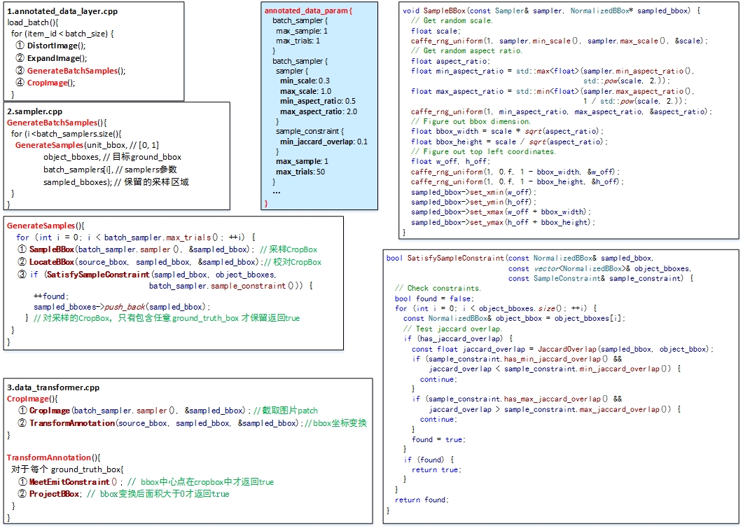
Fig.4 SSD data argument
四. 网络结构
SSD的结构在VGG16网络的基础上进行修改,训练时同样为conv1_1,conv1_2,conv2_1,conv2_2,conv3_1,conv3_2,conv3_3,conv4_1,conv4_2,conv4_3,conv5_1,conv5_2,conv5_3(512),fc6经过3*3*1024的卷积(原来VGG16中的fc6是全连接层,这里变成卷积层,下面的fc7层同理),fc7经过1*1*1024的卷积,conv6_1,conv6_2(对应上图的conv8_2),conv7_1,conv7_2,conv,8_1,conv8_2,conv9_1,conv9_2,loss。然后针对conv4_3(4),fc7(6),conv6_2(6),conv7_2(6),conv8_2(4),conv9_2(4)的每一个再分别采用两个3*3大小的卷积核进行卷积,这两个卷积核是并列的(括号里的数字代表prior box的数量,可以参考Caffe代码,所以上图中SSD结构的倒数第二列的数字8732表示的是所有prior box的数量,是这么来的38*38*4+19*19*6+10*10*6+5*5*6+3*3*4+1*1*4=8732),这两个3*3的卷积核一个是用来做localization的(回归用,如果prior box是6个,那么就有6*4=24个这样的卷积核,卷积后map的大小和卷积前一样,因为pad=1,下同),另一个是用来做confidence的(分类用,如果prior box是6个,VOC的object类别有20个,那么就有6*(20+1)=126个这样的卷积核)。如下图是conv6_2的localizaiton的3*3卷积核操作,卷积核个数是24(6*4=24,由于pad=1,所以卷积结果的map大小不变,下同):这里的permute层就是交换的作用,比如你卷积后的维度是32×24×19×19,那么经过交换层后就变成32×19×19×24,顺序变了而已。而flatten层的作用就是将32×19×19×24变成32*8664,32是batchsize的大小。
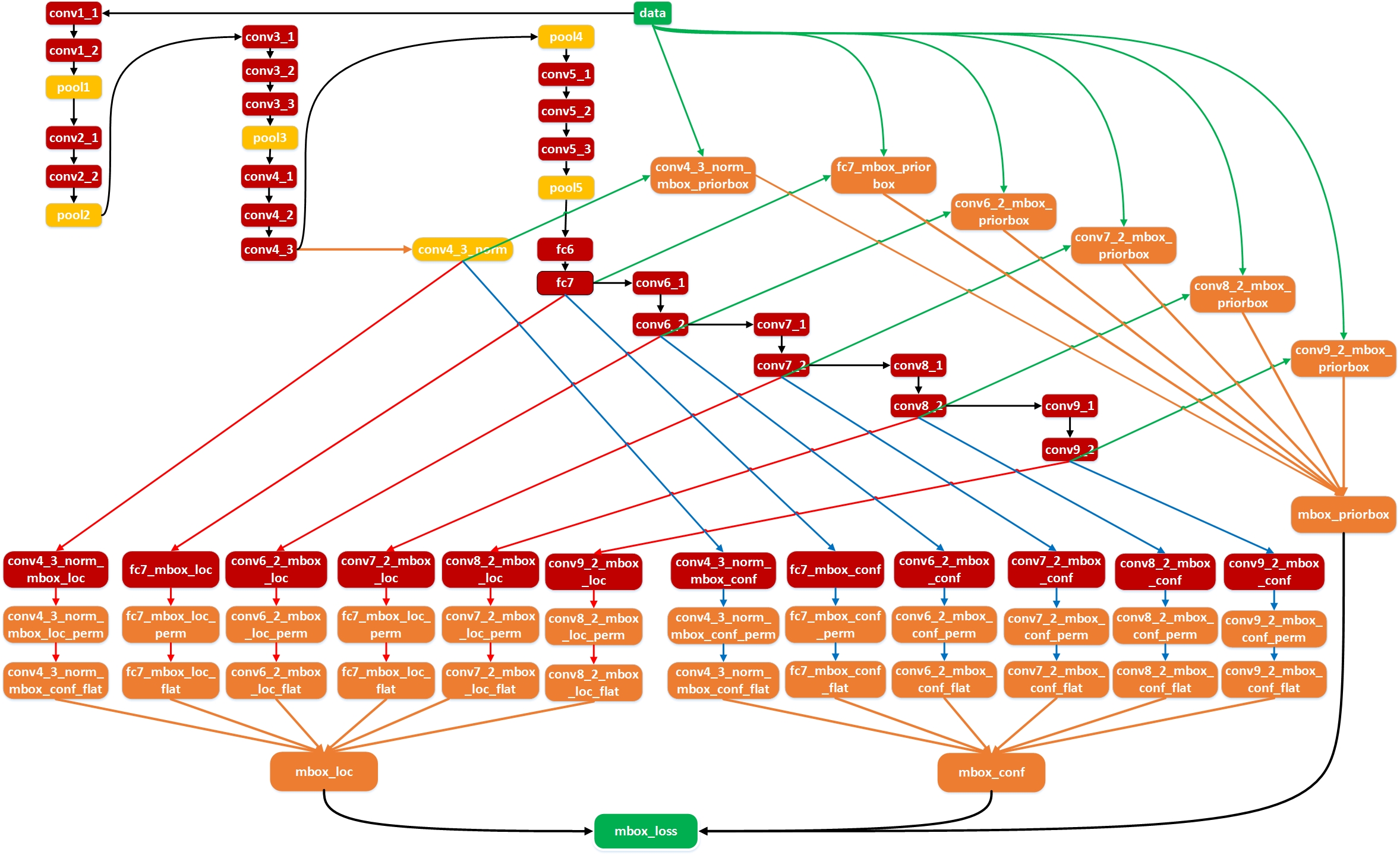
Fig.5 SSD 流程
SSD 网络中输入图片尺寸是3×300×300,经过pool5层后输出为512×19×19,接下来经过fc6(改成卷积层)
layer {
  name: "fc6"
  type: "Convolution"
  bottom: "pool5"
  top: "fc6"
  param {
    lr_mult: 1.0
    decay_mult: 1.0
  }
  param {
    lr_mult: 2.0
    decay_mult: 0.0
  }
  convolution_param {
    num_output: 1024
    pad: 6
    kernel_size: 3
    weight_filler {
      type: "xavier"
    }
    bias_filler {
      type: "constant"
      value: 0.0
    }
    dilation: 6
  }
}
这里来简单提下卷积和池化层前后尺寸的变化:
公式如下,其中,input代表height或者width; dilation默认为1,所以默认kernel_extent=kernel:
$output = \frac{(input + 2*pad - kernel\_extern)}{stride} +1$
$kernel\_extern = dilation * (kernel - 1) + 1$
注意:具体计算时,对于无法整除的情况,Convolution向下取整,Pooling向上取整。。
计算下来会得到fc6层的输出维度:1024×19×19,fc7层:1024×19×19,conv6_1:256×19×19,conv6_2:512×10×10,conv7_1:128×10×10,conv7_2:256×5×5,conv8_1:128×5×5,conv8_2:256×3×3,conv9_1:128×3×3,conv9_2:256×1×1。
计算完后,我们来看看用来检测的6个 feature map 的维度:
| feature map | conv4_3 | fc7 | conv6_2 | conv7_2 | conv8_2 | conv9_2 |
| size | 512×38×38 | 1024×19×19 | 512×10×10 | 256×5×5 | 256×3×3 | 256×1×1 |
每个用来检测的特征层,可以使用一系列 convolutional filters,去产生一系列固定大小的 predictions。对于一个大小为$m×n$,具有$p$通道的feature map,使用的 convolutional filters 就是$3×3×p$的kernels。产生的 predictions,要么就是归属类别的一个score,要么就是相对于 prior box coordinate 的 shape offsets。
对于score,经过卷积预测器后的输出维度为(c*k)×m×n,这里c是类别总数,k是该层设定的default box种类(不同层k的取值不同,分别为4,6,6,6,4,4)
layer {
  name: "conv6_2_mbox_conf"
  type: "Convolution"
  bottom: "conv6_2"
  top: "conv6_2_mbox_conf"
  param {
    lr_mult: 1.0
    decay_mult: 1.0
  }
  param {
    lr_mult: 2.0
    decay_mult: 0.0
  }
  convolution_param {
    num_output: 126
    pad: 1
    kernel_size: 3
    stride: 1
    weight_filler {
      type: "xavier"
    }
    bias_filler {
      type: "constant"
      value: 0.0
    }
  }
}
维度变化为:
| layer | conv4_3_norm_mbox_ conf | fc7_mbox_ conf | conv6_2_mbox_ conf | conv7_2_mbox_ conf | conv8_2_mbox_ conf | conv9_2_mbox_ conf |
| size | 84 38 38 | 126 19 19 | 126 10 10 | 126 5 5 | 84 3 3 | 84 1 1 |
最后经过 permute 层交换维度
| layer | conv4_3_norm_mbox_ conf_perm | fc7_mbox_ conf_perm | conv6_2_mbox_ conf_perm | conv7_2_mbox_ conf_perm | conv8_2_mbox_ conf_perm | conv9_2_mbox_ conf_perm |
| size | 38 38 84 | 19 19 126 | 10 10 126 | 5 5 126 | 3 3 84 | 1 1 84 |
最后经过 flatten 层整合
| layer | conv4_3_norm_mbox_ conf_flat | fc7_mbox_ conf_flat | conv6_2_mbox_ conf_flat | conv7_2_mbox_ conf_flat | conv8_2_mbox_ conf_flat | conv9_2_mbox_ conf_flat |
| size | 121296 | 45486 | 12600 | 3150 | 756 | 84 |
对于offset,经过卷积预测器后的输出值为(4*k)×m×n,这里4是(x,y,w,h),k是该层设定的prior box数量(不同层k的取值不同,分别为4,6,6,6,4,4):
layer {
  name: "conv6_2_mbox_loc"
  type: "Convolution"
  bottom: "conv6_2"
  top: "conv6_2_mbox_loc"
  param {
    lr_mult: 1.0
    decay_mult: 1.0
  }
  param {
    lr_mult: 2.0
    decay_mult: 0.0
  }
  convolution_param {
    num_output: 24
    pad: 1
    kernel_size: 3
    stride: 1
    weight_filler {
      type: "xavier"
    }
    bias_filler {
      type: "constant"
      value: 0.0
    }
  }
}
维度变化为:
| layer | conv4_3_norm_mbox_ loc | fc7_mbox_ loc | conv6_2_mbox_ loc | conv7_2_mbox_ loc | conv8_2_mbox_ loc | conv9_2_mbox_ loc |
| size | 16 38 38 | 24 19 19 | 24 10 10 | 24 5 5 | 16 3 3 | 16 1 1 |
随后经过 permute 层交换维度
| layer | conv4_3_norm_mbox_ loc_perm | fc7_mbox_ loc_perm | conv6_2_mbox_ loc_perm | conv7_2_mbox_ loc_perm | conv8_2_mbox_ loc_perm | conv9_2_mbox_ loc_perm |
| size | 38 38 16 | 19 19 24 | 10 10 24 | 5 5 24 | 3 3 16 | 1 1 16 |
最后经过 flatten 层整合
| layer | conv4_3_norm_mbox_ loc_flat | fc7_mbox_ loc_flat | conv6_2_mbox_ loc_flat | conv7_2_mbox_ loc_flat | conv8_2_mbox_ loc_flat | conv9_2_mbox_ loc_flat |
| size | 23104 | 8664 | 2400 | 600 | 144 | 16 |
同时,各个feature map层经过priorBox层生成prior box
生成prior box的操作:根据最小尺寸 scale以及横纵比aspect ratio按照步长step生成,step表示该层的一个像素点相当于输入图像里的尺寸,简单讲就是感受野,源码里面是通过将原始的 input image的大小除以该层 feature map的大小来得到的。variance是一个尺度变换因子,本文的四个坐标采用的是中心坐标加上长宽,计算loss的时候可能需要对中心坐标的loss和长宽的loss做一个权衡,所以有了这个variance。如果采用的是box的四大顶点坐标这种方式,默认variance都是0.1,即相互之间没有权重差异。It is used to encode the ground truth box w.r.t. the prior box. You can check this function. Note that it is used in the original MultiBox paper by Erhan etal. It is also used in Faster R-CNN as well. I think the major goal of including the variance is to scale the gradient. Of course you can also think of it as approximate a gaussian distribution with variance of 0.1 around the box coordinates.
layer {
  name: "conv6_2_mbox_priorbox"
  type: "PriorBox"
  bottom: "conv6_2"
  bottom: "data"
  top: "conv6_2_mbox_priorbox"
  prior_box_param {
    min_size: 111.0
    max_size: 162.0
    aspect_ratio: 2.0
    aspect_ratio: 3.0
    flip: true
    clip: false
    variance: 0.10000000149
    variance: 0.10000000149
    variance: 0.20000000298
    variance: 0.20000000298
    step: 32.0
    offset: 0.5
  }
}
维度变化为:
| layer | conv4_3_norm_mbox_ priorbox | fc7_mbox_ priorbox | conv6_2_mbox_ priorbox | conv7_2_mbox_ priorbox | conv8_2_mbox_ priorbox | conv9_2_mbox_ priorbox |
| size | 2 23104 | 2 8664 | 2 2400 | 2 600 | 2 144 | 2 16 |
经过上述3个操作后,对每一层feature的处理就结束了。
对前面所列的5个卷积层输出都执行上述的操作后,就将得到的结果合并:采用Concat,类似googleNet的Inception操作,是通道合并而不是数值相加。
layer {
  name: "mbox_loc"
  type: "Concat"
  bottom: "conv4_3_norm_mbox_loc_flat"
  bottom: "fc7_mbox_loc_flat"
  bottom: "conv6_2_mbox_loc_flat"
  bottom: "conv7_2_mbox_loc_flat"
  bottom: "conv8_2_mbox_loc_flat"
  bottom: "conv9_2_mbox_loc_flat"
  top: "mbox_loc"
  concat_param {
    axis: 1
  }
}
layer {
  name: "mbox_conf"
  type: "Concat"
  bottom: "conv4_3_norm_mbox_conf_flat"
  bottom: "fc7_mbox_conf_flat"
  bottom: "conv6_2_mbox_conf_flat"
  bottom: "conv7_2_mbox_conf_flat"
  bottom: "conv8_2_mbox_conf_flat"
  bottom: "conv9_2_mbox_conf_flat"
  top: "mbox_conf"
  concat_param {
    axis: 1
  }
}
layer {
  name: "mbox_priorbox"
  type: "Concat"
  bottom: "conv4_3_norm_mbox_priorbox"
  bottom: "fc7_mbox_priorbox"
  bottom: "conv6_2_mbox_priorbox"
  bottom: "conv7_2_mbox_priorbox"
  bottom: "conv8_2_mbox_priorbox"
  bottom: "conv9_2_mbox_priorbox"
  top: "mbox_priorbox"
  concat_param {
    axis: 2
  }
}
这是几个通道合并后的维度:
| layer | mbox_loc | mbox_conf | mbox_priorbox |
| size | 34928(8732*4) | 183372(8732*21) | 2 34928(8732*4) |
最后就是作者自定义的损失函数层,这里的overlap_threshold表示prior box和ground truth的重合度超过这个阈值则为正样本。另外我觉得具体哪些prior box是正样本,哪些是负样本是在loss层计算出来的,不过这个细节与算法关系不大:
layer {
  name: "mbox_loss"
  type: "MultiBoxLoss"
  bottom: "mbox_loc"
  bottom: "mbox_conf"
  bottom: "mbox_priorbox"
  bottom: "label"
  top: "mbox_loss"
  include {
    phase: TRAIN
  }
  propagate_down: true
  propagate_down: true
  propagate_down: false
  propagate_down: false
  loss_param {
    normalization: VALID
  }
  multibox_loss_param {
    loc_loss_type: SMOOTH_L1
    conf_loss_type: SOFTMAX
    loc_weight: 1.0
    num_classes: 21
    share_location: true
    match_type: PER_PREDICTION
    overlap_threshold: 0.5
    use_prior_for_matching: true
    background_label_id: 0
    use_difficult_gt: true
    neg_pos_ratio: 3.0
    neg_overlap: 0.5
    code_type: CENTER_SIZE
    ignore_cross_boundary_bbox: false
    mining_type: MAX_NEGATIVE
  }
}
损失函数方面:和Faster RCNN的基本一样,由分类和回归两部分组成,可以参考Faster RCNN,这里不细讲。总之,回归部分的loss是希望预测的box和prior box的差距尽可能跟ground truth和prior box的差距接近,这样预测的box就能尽量和ground truth一样。

上面得到的8732个目标框经过Jaccard Overlap筛选剩下几个了;其中不满足的框标记为负数,其余留下的标为正数框。紧随其后:
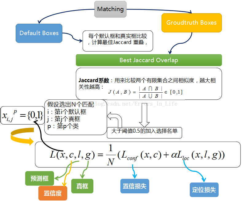
训练过程中的 prior boxes 和 ground truth boxes 的匹配,基本思路是:让每一个 prior box 回归并且到 ground truth box,这个过程的调控我们需要损失层的帮助,他会计算真实值和预测值之间的误差,从而指导学习的走向。
SSD 训练的目标函数(training objective)源自于 MultiBox 的目标函数,但是本文将其拓展,使其可以处理多个目标类别。具体过程是我们会让每一个 prior box 经过Jaccard系数计算和真实框的相似度,阈值只有大于 0.5 的才可以列为候选名单;假设选择出来的是N个匹配度高于百分之五十的框吧,我们令 i 表示第 i 个默认框,j 表示第 j 个真实框,p表示第p个类。那么$x_{ij}^p$表示 第 i 个 prior box 与 类别 p 的 第 j 个 ground truth box 相匹配的Jaccard系数,若不匹配的话,则$x_{ij}^p=0$。总的目标损失函数(objective loss function)就由 localization loss(loc) 与 confidence loss(conf) 的加权求和:
- N 是与 ground truth box 相匹配的 prior boxes 个数
- localization loss(loc) 是 Fast R-CNN 中 Smooth L1 Loss,用在 predict box(l) 与 ground truth box(g) 参数(即中心坐标位置,width、height)中,回归 bounding boxes 的中心位置,以及 width、height
- confidence loss(conf) 是 Softmax Loss,输入为每一类的置信度 c
- 权重项 α,可在protxt中设置 loc_weight,默认设置为 1
五. 代码
代码很多,想快速SSD算法只需要详细了解下它的样本增广、正负样本获取方式、损失函数这三个方面就好,主要包括 include/caffe/ 目录下面的 annotated_data_layer.hpp 、 detection_evaluate_layer.hpp 、 detection_output_layer.hpp 、 multibox_loss_layer.hpp 、 prior_box_layer.hpp ,以及对应的 src/caffe/layers/ 目录下面的cpp和cu文件,另外还有 src/caffe/utlis/ 目录下面的 bbox_util.cpp 。从名字就可以看出来, annotated_data_layer 是提供数据的、 detection_evaluate_layer 是验证模型效果用的、 detection_output_layer 是输出检测结果用的、 multibox_loss_layer 是loss、 prior_box_layer 是计算prior bbox的。
annotated_data_layer.cpp sampler.cpp data_transformer.cpp
这部分代码涉及到样本读取和data augment,同时把每张图里的groundtruth bbox读出来传给下一层。从 load_batch() 函数开始,主要包含四个部分,具体见上面一个图
① DistortImage();
② ExpandImage();
③ GenerateBatchSamples();
④ CropImage();
prior_box_layer.cpp
这一层完成的是给定一系列feature map后如何在上面生成prior box。从函数 Forward_cpu() 函数开始。SSD的做法很有意思,对于输入大小是 W×H 的feature map,生成的prior box中心就是 W×H 个,均匀分布在整张图上,像下图中演示的一样。在每个中心上,可以生成多个不同长宽比的prior box,如[1/3, 1/2, 1, 2, 3]。所以在一个feature map上可以生成的prior box总数是 W×H×length_of_aspect_ratio ,对于比较大的feature map,如VGG的conv4_3,生成的prior box可以达到数千个。当然对于边界上的box,还要做一些处理保证其不超出图片范围,这都是细节了。
这里需要注意的是,虽然prior box的位置是在 W×H 的格子上,但prior box的大小并不是跟格子一样大,而是人工指定的,原论文中随着feature map从底层到高层,prior box的大小在0.2到0.9之间均匀变化。
multibox_loss_layer.cpp
FindMatches()
我们已经在图上画出了prior box,同时也有了ground truth,那么下一步就是将prior box匹配到ground truth上,这是在
src/caffe/utlis/bbox_util.cpp的FindMatches函数里完成的。值得注意的是这里不光是给每个groudtruth box找到了最匹配的prior box,而是给每个prior box都找到了匹配的groundtruth box(如果有的话),这样显然大大增大了正样本的数量。
MineHardExamples()
给每个prior box找到匹配(包括物体和背景)之后,似乎可以定义一个损失函数,给每个prior box标记一个label,扔进去一通训练。
但需要注意的是,任意一张图里负样本一定是比正样本多得多的,这种严重不平衡的数据会严重影响模型的性能,所以对负样本要有所选择。
这里简单描述下:假设我们上一步得到了N个负样本,接下来我们将 loc_pred 损失进行排序,选择 N 个最大的 loc_pred 保留下来。然后只将索引存在于 loc_pred 里的 负样本留下来。
EncodeLocPrediction() && EncodeConfPrediction ()
因为我们对prior box是有选择的,所以数据的形状在这里已经被打乱了,没办法直接在后面连接一个loss(Caffe等框架需要每一层的输入是四维张量),
所以需要我们把选出来的数据重新整理一下,这一步是在
src/caffe/utlis/bbox_util.cpp的EncodeLocPrediction和EncodeConfPrediction两个函数里完成的。
六.使用注意
1. 使用batch_sampler做data argument时要注意是否crop的样本只包含目标很小一部分。
2.检查对于你的样本来说回归和分类问题哪个更难,以此调整multibox_loss_param中loc_weight进行训练。
3.正负样本比例,默认HARD_EXAMPLE方式只取64个最高predictions loss来从中寻找负样本,检查你的样本集中正负样本比例是否合适。


 805
805


 被折叠的 条评论
为什么被折叠?
被折叠的 条评论
为什么被折叠?
 到【灌水乐园】发言


