期末大作业

 

一、boston房价预测

1. 读取数据集

2. 训练集与测试集划分

3. 线性回归模型：建立13个变量与房价之间的预测模型，并检测模型好坏。

4. 多项式回归模型：建立13个变量与房价之间的预测模型，并检测模型好坏。

 

#1. 读取数据集
from sklearn.datasets import load_boston
data = load_boston()

#2. 训练集与测试集划分
from sklearn.model_selection import train_test_split
x_train, x_test, y_train, y_test= train_test_split(data.data,data.target,test_size=0.3)

#3. 线性回归模型：建立13个变量与房价之间的预测模型，并检测模型好坏。
from sklearn.linear_model import LinearRegression
mlr = LinearRegression()
mlr.fit(x_train,y_train)
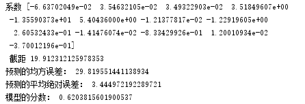
print('系数',mlr.coef_,"\n","截距",mlr.intercept_)
from sklearn.metrics import regression
y_pred = mlr.predict(x_test)
print("预测的均方误差：", regression.mean_squared_error(y_test,y_pred))
print("预测的平均绝对误差：", regression.mean_absolute_error(y_test,y_pred))
print("模型的分数：",mlr.score(x_test, y_test))

#4. 多项式回归模型：建立13个变量与房价之间的预测模型，并检测模型好坏。
from sklearn.preprocessing import PolynomialFeatures
a = PolynomialFeatures(degree=2)
x_poly_train = a.fit_transform(x_train)
x_poly_test = a.transform(x_test)
mlrp = LinearRegression()
mlrp.fit(x_poly_train, y_train)
y_pred2 = mlrp.predict(x_poly_test)
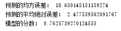
print("预测的均方误差：", regression.mean_squared_error(y_test,y_pred2))
print("预测的平均绝对误差：", regression.mean_absolute_error(y_test,y_pred2))
print("模型的分数：",mlrp.score(x_poly_test, y_test))

　　

 

5. 比较线性模型与非线性模型的性能，并说明原因。

非线性模型，即多项式回归模型性能较好，因为它是有很多点连接而成的曲线，对样本的拟合程度较高，预测效果误差较小

 

二、中文文本分类

按学号未位下载相应数据集。

147：财经、彩票、房产、股票、

258：家居、教育、科技、社会、时尚、

0369：时政、体育、星座、游戏、娱乐

分别建立中文文本分类模型，实现对文本的分类。基本步骤如下：

1.各种获取文件，写文件

2.除去噪声，如：格式转换，去掉符号，整体规范化

3.遍历每个个文件夹下的每个文本文件。

4.使用jieba分词将中文文本切割。

中文分词就是将一句话拆分为各个词语，因为中文分词在不同的语境中歧义较大，所以分词极其重要。

可以用jieba.add_word('word')增加词，用jieba.load_userdict('wordDict.txt')导入词库。

维护自定义词库

5.去掉停用词。

维护停用词表

6.对处理之后的文本开始用TF-IDF算法进行单词权值的计算

7.贝叶斯预测种类

8.模型评价

9.新文本类别预测

 

处理过程中注意：

• 实验过程中文件遍历从少量到多量，调试无误后再处理全部文件
• 判断文件大小决定读取方法
• 注意保存中间结果，以免每次从头读取文件重复处理
• 内存不足时进行分批处理
• 利用数组的保存np.save('x1.npy',x1)与数组的读取np.load('x1.npy')和数组的拼接np.concatenate((x1,x2),axis=0)
• 及时用 del(x1) 释放大块内存，用gc.collect()回收内存。
• 边处理边保存数据，不要处理完了一次性保存。万一中间发生的异常情况，就全部白做了。
• 进行Python 异常处理，把出错的文件单独记录，程序可以继续执行。回头再单独处理出错的文件。
• 在准备长时间无监督运行程序之前，请关闭windows自动更新、自动屏保关机等......

import os
import numpy as np
import sys
from datetime import datetime
import gc
path = 'G:\\258'

# 导入结巴库，并将需要用到的词库加进字典
import jieba
jieba.load_userdict('jiaju.txt')
# 导入停用词：
with open(r'stopsCN.txt', encoding='utf-8') as f:
    stopwords = f.read().split('\n')

def processing(tokens):
    # 去掉非字母汉字的字符
    tokens = "".join([char for char in tokens if char.isalpha()])
    # 结巴分词
    tokens = [token for token in jieba.cut(tokens,cut_all=True) if len(token) >=2]
    # 去掉停用词
    tokens = " ".join([token for token in tokens if token not in stopwords])
    return tokens


# 用os.walk获取需要的变量，并拼接文件路径再打开每一个文件
tokenList = []
targetList = []
for root,dirs,files in os.walk(path):
    for f in files:
        filePath = os.path.join(root,f)#地址拼接
        with open(filePath, encoding='utf-8') as f:
            content = f.read()
            # 获取类别标签，并处理该新闻
        target = filePath.split('\\')[-2]
        targetList.append(target)
        tokenList.append(processing(content))



# 划分训练集测试集并建立特征向量,为建立模型做准备
# 划分训练集测试集
from sklearn.feature_extraction.text import TfidfVectorizer
from sklearn.model_selection import train_test_split
from sklearn.naive_bayes import GaussianNB,MultinomialNB
from sklearn.model_selection import cross_val_score
from sklearn.metrics import classification_report
x_train,x_test,y_train,y_test = train_test_split(tokenList,targetList,test_size=0.2,stratify=targetList)
# 转化为特征向量，这里选择TfidfVectorizer的方式建立特征向量。不同新闻的词语使用会有较大不同。
vectorizer = TfidfVectorizer()
X_train = vectorizer.fit_transform(x_train)
X_test = vectorizer.transform(x_test)
# 建立模型,这里用多项式朴素贝叶斯，因为样本特征的a分布大部分是多元离散值
mnb = MultinomialNB()
module = mnb.fit(X_train, y_train)

#进行预测
y_predict = module.predict(X_test)
# 输出模型精确度
scores=cross_val_score(mnb,X_test,y_test,cv=5)
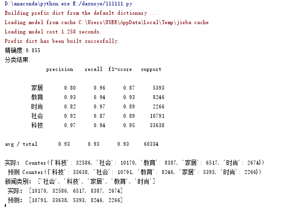
print("精确度:%.3f"%scores.mean())
# 输出模型评估报告
print("分类结果:\n",classification_report(y_predict,y_test))


# 将预测结果和实际结果进行对比
# 统计测试集和预测集的各类新闻个数
import collections
testCount = collections.Counter(y_test)
predCount = collections.Counter(y_predict)
print('实际：',testCount,'\n', '预测', predCount)

# 建立标签列表，实际结果列表，预测结果列表，
nameList = list(testCount.keys())
testList = list(testCount.values())
predictList = list(predCount.values())
x = list(range(len(nameList)))
print("文本类别：",nameList,'\n',"实际：",testList,'\n',"预测：",predictList)

# 画图
import matplotlib.pyplot as plt
from pylab import mpl
mpl.rcParams['font.sans-serif'] = ['FangSong'] # 指定默认字体
plt.figure(figsize=(7,5))
total_width, n = 0.6, 2
width = total_width / n
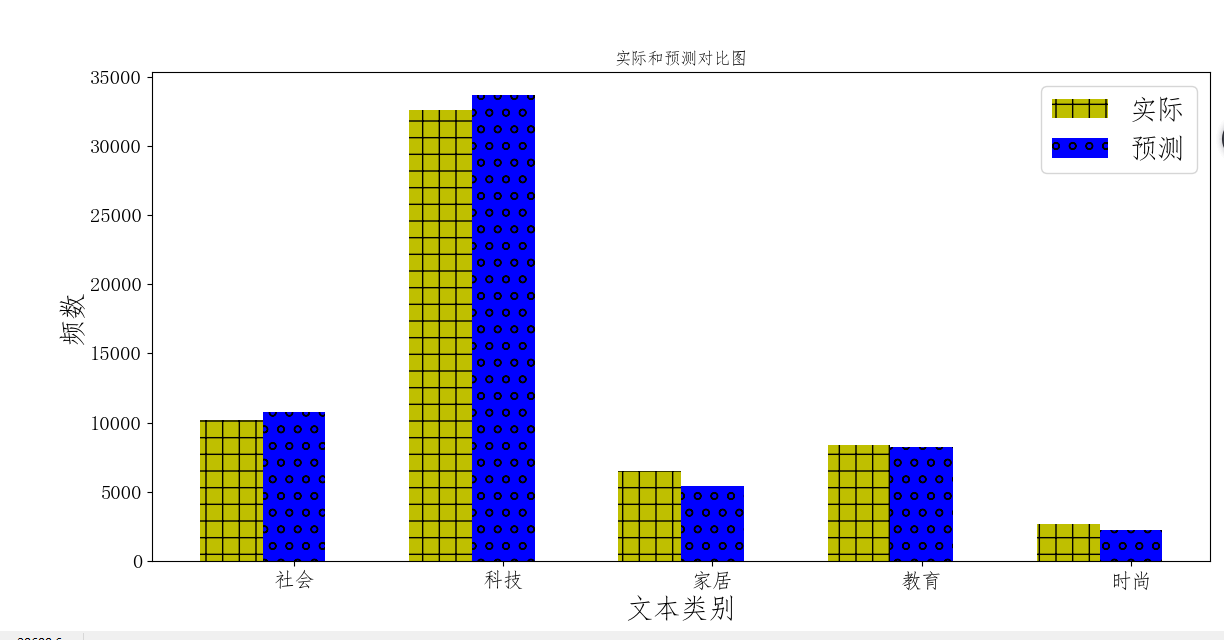
plt.bar(x, testList, width=width,label='实际',facecolor = 'y',hatch = '+')
for i in range(len(x)):
    x[i] = x[i] + width
plt.bar(x, predictList,width=width,label='预测',tick_label = nameList,facecolor='b',hatch = 'o')
plt.title('实际和预测对比图',fontsize=20)
plt.xlabel('文本类别',fontsize=20)
plt.ylabel('频数',fontsize=20)
plt.legend(fontsize =20)
plt.tick_params(labelsize=15)
plt.show()

　

 

 

 

转载于:https://www.cnblogs.com/ljy28/p/10153509.html