Half Wavelength Dipole Antenna

Reference :

1. wikipedia

The dipole antenna is the simplest and most widely used class of antenna.It consists of two identical conductive elements such as metal wires or rods, which are usually bilaterally symmetrical.Each side of the feedline to the transmitter or receiver is connected to one of the conductors.

Dipoles are resonant antennas, meaning that the elements serve as resonators, with standing waves of radio current flowing back and forth between their ends. So the length of the dipole elements is determined by the wavelength of the radio waves used. The most common form is the half-wave dipole, in which each of the two rod elements is approximately 1/4 wavelength long, so the whole antenna is a half-wavelength long. The radiation pattern of a vertical dipole is omnidirectional; it radiates equal power in allazimuthal directions perpendicular to the axis of the antenna. For a half-wave dipole the radiation is maximum, 2.15 dBi perpendicular to the antenna axis, falling monotonically with elevation angle to zero on the axis, off the ends of the antenna.

Several different variations of the dipole are also used, such as thefolded dipole, short dipole, cage dipole, bow-tie, and batwing antenna. Dipoles may be used as standalone antennas themselves, but they are also employed as feed antennas (driven elements) in many more complex antenna types, such as the Yagi antenna, parabolic antenna, reflective array, turnstile antenna, log periodic antenna, and phased array.

Dipole characteristics

 

1. Impedance

The feedpoint impedance of a dipole antenna is very sensitive to its electrical length. Therefore, a dipole will generally only perform optimally over a rather narrow bandwidth, beyond which its impedance will become a poor match for the transmitter or receiver (and transmission line). The real (resistive) and imaginary (reactive) components of that impedance, as a function of electrical length, are shown in the accompanying graph.

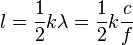
A true half-wave dipole is one half of the wavelength λ in length, where λ=c/f in free space. Such a dipole has a feedpoint impedance consisting of 73Ω resistance and +43Ω reactance, thus presenting a slightly inductive reactance. In order to cancel that reactance, and present a pure resistance to the feedline, the element is shortened by the factor k for a net length of:

The adjustment factor k, in order for the reactance to be cancelled, depends on the diameter of the conductor. For thin wires (diameter= 0.00001 wavelengths), k is approximately 0.98; for thick conductors (diameter= 0.008 wavelengths), k drops to about 0.94. This is because the effect of antenna length on reactance is much greater for thinner conductors. For the same reason, antennas with thicker conductors have a wider operating bandwidth over which they attain an acceptablestanding wave ratio.

Dipole antennas of lengths approximately equal to any odd multiple of λ/2 are also resonant, presenting a small reactance (which can be cancelled by a small length adjustment). However these are rarely used. One size that is more practical though is a dipole with a length of 5/4 wavelengths. Not being close to 3/2 wavelengths, this antenna's impedance has a large (negative) reactance and can only be used with an impedance matching network (or "antenna tuner"). It is a desirable length because such an antenna has the highest gain for any dipole which isn't a great deal longer.

2. Radiation pattern and gain

Neglecting electrical inefficiency, the antenna gain is equal to the directive gain, which is 1.5 or 1.76 dBi for a short dipole, increasing to 1.64 or 2.15 dBi for a half-wave dipole. For a 5/4 wave dipole the gain further increases to about 5.2 dBi, making this length desirable for that reason even though the antenna is then off-resonance. Longer dipoles than that have radiation patterns that are multi-lobed, with poorer gain (unless they are much longer) even along the strongest lobe.

3. Feeding a dipole antenna

Ideally, a half-wave dipole should be fed using a balanced transmission line matching its typical 65 - 70Ω input impedance. Twin lead with a similar impedance is available but seldom used.

Many types of coaxial cable have a characteristic impedance of 75Ω, which would therefore be a good match for a half-wave dipole, however coax is an unbalanced transmission line (with one terminal at ground potential) whereas a dipole antenna presents a balanced input (both terminals have an equal but opposite voltage with respect to ground). When a balanced antenna is fed with a single-ended line, common mode currents can cause the coax line to radiate in addition to the antenna itself, distorting the radiation pattern and changing the impedance seen by the line. The dipole can be properly fed, and retain its expected characteristics, by using a balun in between the coaxial feedline and the antenna terminals. Connection of coax to a dipole antenna using a balun is plot  below.

Another solution, especially for receiving antennas, is to use common 300 ohm twin lead in conjunction with a folded dipole. The folded dipole is similar to the simple half-wave dipole but with the feedpoint impedance multiplied by 4, thus closely matching that 300 ohm impedance. This is the most common household antenna for fixed FM broadcast band tuners, which usually include balanced 300 ohm antenna input terminals.

^{4. detailed calculation}

The current distribution is that of a standing wave, approximately sinusoidal along the length of the dipole, with a node at each end and an antinode (peak current) at the center (feedpoint):

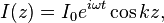
where k = 2π/λ and z runs from −L /2 to L /2.

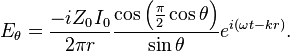
In the far field, this produces a radiation pattern whose electric field is given by

A numerical integration of this integral over all solid angle, as we did for the short dipole, supplies a value for the radiation resistance: Using the induced EMF method, the real part of the driving point impedance can also be written in terms of the cosine integral:

 

5 simlation result

转载于:https://www.cnblogs.com/hiramlee0534/p/5296755.html