AI-CSP:definition, Constraint propagation, Backtracking search, Local search, problem structure.

Define CSP

 

CSPs represent a state with a set of variable/value pairs and represent the conditions for a solution by a set of constraints on the variables. Many important real-world problems can be described as CSPs.

 

CSP (constraint satisfaction problem): Use a factored representation (a set of variables, each of which has a value) for each state, a problem that is solved when each variable has a value that satisfies all the constraints on the variable is called a CSP.

 

A CSP consists of 3 components:

 

·X is a set of variables, {X₁, …, X_n}.

 

·D is a set of domains, {D₁, …, D_n}, one for each variable.

 

Each domain D_i consists of a set of allowable values, {v₁, …, v_k} for variable X_i.

 

·C is a set of constraints that specify allowable combination of values.

 

Each constraint C_i consists of pair <scope, rel>, where scope is a tuple of variables that participate in the constraint, and rel is a relation that defines the values that those variables can take on.

 

A relation can be represented as: a. an explicit list of all tuples of values that satisfy the constraint; or b. an abstract relation that supports two operations. (e.g. if X₁ and X₂ both have the domain {A,B}, the constraint saying “the two variables must have different values” can be written as a. <(X₁,X₂),[(A,B),(B,A)]> or b. <(X₁,X₂),X₁≠X₂>.

 

Assignment:

 

Each state in a CSP is defined by an assignment of values to some of the variables, {X_i=v_i, X_j=v_j, …};

 

An assignment that does not violate any constraints is called a consistent or legal assignment;

 

A complete assignment is one in which every variable is assigned;

 

A solution to a CSP is a consistent, complete assignment;

 

A partial assignment is one that assigns values to only some of the variables.

 

 

 

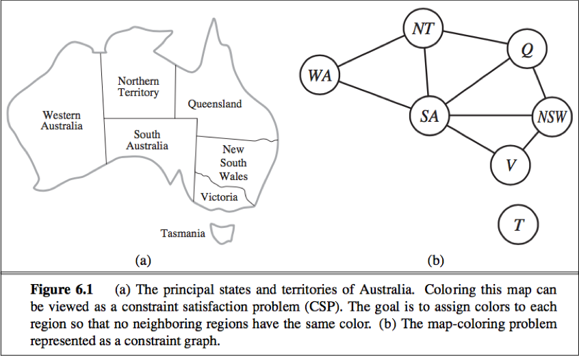
Map coloring

 

To formulate a CSP:

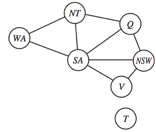
define the variables to be the regions X = {WA, NT, Q, NSW, V, SA, T}.

The domain of each variable is the set D_i = {red, green, blue}.

The constraints is C = {SA≠WA, SAW≠NT, SA≠Q, SA≠NSW, SA≠V, WA≠NT, NT≠Q, Q≠NSW, NSW≠V}. ( SA≠WA is a shortcut for <(SA,WA),SA≠WA>. )

Constraint graph: The nodes of the graph correspond to variables of the problem, and a link connects to any two variables that participate in a constraint.

 

Advantage of formulating a problem as a CSP:

1) CSPs yield a natural representation for a wide variety of problems;

2) CSP solvers can be faster than state-space searchers because the CSP solver can quickly eliminate large swatches of the search space;

3) With CSP, once we find out that a partial assignment is not a solution, we can immediately discard further refinements of the partial assignment.

4) We can see why a assignment is not a solution—which variables violate a constraint.

 

Job-shop scheduling

Consider a small part of the car assembly, consisting of 15 tasks: install axles (front and back), affix all four wheels (right and left, front and back), tighten nuts for each wheel, affix hubcaps, and inspect the final assembly. Represent the tasks with 15 variables:

X = {Axle_F, Axle_B, Wheel_RF, Wheel_LF, Wheel_RB, Wheel_LB, Nuts_RF, Nuts_LF, Nuts_RB, Nuts_LB, Cap_RF, Cap_LF, Cap_RB, Cap_LB, Inspect}. The value of each variable is the time that the task starts.

Precedent constraints: Whenever a task T₁ must occur before task T₂, and T₁ take duration d₁ to complete. We add an arithmetic constraint of the form T₁ + d₁ ≤ T₂ . So,

 Axle_F + 10 ≤ Wheel_RF ; Axle_F + 10 ≤ Wheel_LF ; Axle_B + 10 ≤ Wheel_RB ; Axle_B + 10 ≤ Wheel_LB ;

Wheel_RF + 1 ≤ Nuts_RF ; Wheel_LF + 1 ≤ Nuts_LF ; Wheel_RB + 1 ≤ Nuts_RB ; Wheel_LB + 1 ≤ Nuts_LB ;

Nuts_RF + 2 ≤ Cap_RF ; Nuts_LF + 2 ≤ Cap_LF ; Nuts_RB + 2 ≤ Cap_RB ; Nuts_LB + 2 ≤ Cap_LB;

Disjunctive constraint: Axle_F and Axle_B must not overlap in time. So,

( Axle_F + 10 ≤ Axle_B ) or ( Axle_B + 10 ≤ Axle_F )

Assert that the inspection come last and takes 3 minutes. For every variable except Inspect we add a constraint of the form X + d_X ≤ Inspect.

There is a requirement to get the whle assembly done in 30 minutes, we can achieve that by limiting the domain of all variables:

Di = {1, 2, 3, …, 27}.

 

Variation on the CSP formalism

a. Types of variables in CSPs

The simplest kind of CSP involves variables that have discrete, finite domains. E.g. Map-coloring problems, scheduling with time limits, the 8-queens problem.

A discrete domain can be infinite. e.g. The set of integers or strings. With infinite domains, to describe constraints, a constraint language must be used instead of enumerating all allowed combinations of values.

CSP with continuous domains are common in the real world and are widely studied in the field of operations research.

The best known category of continuous-domain CSPs is that of linear programming problems, where constraints must be linear equalities or inequalities. Linear programming problems can be solved in time polynomial in the number of variables.

b. Types of constraints in CSPs

The simplest type is the unary constraint, which restricts the value of a single variable.

A binary constraint relates two variables. (e.g. SA≠NSW.) A binary CSP is one with only binary constraints, can be represented as a constraint graph.

We can also describe higher-order constraints. (e.g. The ternary constraint Between(X, Y, Z).)

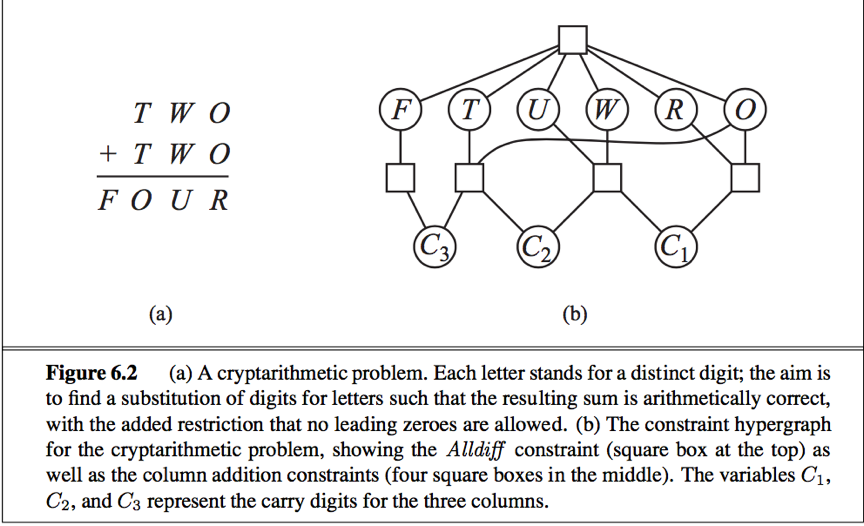
A constraint involving an arbitrary number of variables is called a global constraint. (Need not involve all the variable in a problem.) One of the most common global constraint is Alldiff, which says that all of the variables involved in the constraint must have different values.

Constraint hypergraph: consists of ordinary nodes (circles in the figure) and hypernodes (the squares), which represent n-ary constraints.

Two ways to transform an n-ary CSP to a binary one:

a. Every finite domain constraint can be reduced to a set of binary constraints if enough auxiliary variables are introduced, so we could transform any CSP into one with only binary constraints.

b. The dual-graph transformation: create a new graph in which there will be one variable for each constraint in the original graph, and one binary constraint for each pair of constraints in the original graph that share variables.

e.g. If the original graph has variable {X,Y,Z} and constraints <(X,Y,Z),C₁> and <(X,Y),C₂>, then the dual graph would have variables {C₁,C₂} with the binary constraint <(X,Y),R₁>, where (X,Y) are the shared variables and R₁ is a new relation that defines the constraint between the shared variables.

 

We might prefer a global constraint (such as Alldiff) rather than a set of binary constraints for two reasons:

1) easier and less error-prone to write the problem description.

2) possible to design special-purpose inference algorithms for global constraints that are not available for a set of more primitive constraints.

 

Absolute constraints: Violation of which rules out a potential solution.

Preference constraints: indicate which solutions are preferred, included in many real-world CSPs. Preference constraints can often be encoded as costs on individual variable assignments, with this formulation, CSPs with preferences can be solved with optimization search methods. We ca call such a problem a constraint optimization problem(COP). Linear programming problems do this kind of optimization.

 

Constraint propagation: Inference in CSPs

A number of inference techniques use the constraints to infer which variable/value pairs are consistent and which are not. These include node, arc, path, and k-consistent.

constraint propagation: Using the constraints to reduce the number of legal values for a variable, which in turn can reduce the legal values for another variable, and so on.

local consistency: If we treat each variable as a node in a graph and each binary constraint as an arc, then the process of enforcing local consistency in each part of the graph causes inconsistent values to be eliminated throughout the graph.

There are different types of local consistency:

Node consistency

A single variable (a node in the CSP network) is node-consistent if all the values in the variable’s domain satisfy the variable’s unary constraint.

We say that a network is node-consistent if every variable in the network is node-consistent.

 

Arc consistency

A variable in a CSP is arc-consistent if every value in its domain satisfies the variable’s binary constraints.

X_i is arc-consistent with respect to another variable X_j if for every value in the current domain D_i there is some value in the domain D_j that satisfies the binary constraint on the arc (X_i, X_j).

A network is arc-consistent if every variable is arc-consistent with every other variable.

Arc consistency tightens down the domains (unary constraint) using the arcs (binary constraints).

AC-3 algorithm:

 

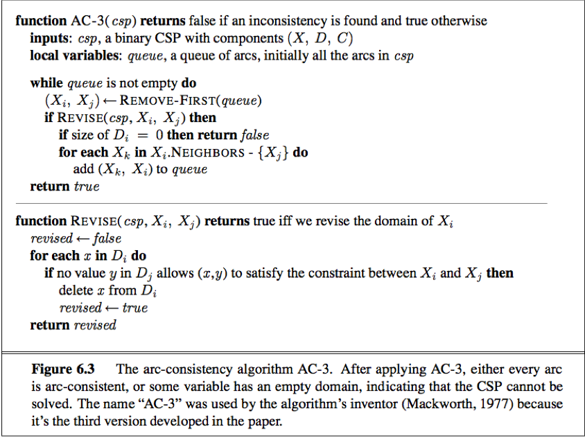
AC-3 maintains a queue of arcs which initially contains all the arcs in the CSP.

AC-3 then pops off an arbitrary arc (X_i, X_j) from the queue and makes X_i arc-consistent with respect to X_j.

If this leaves D_i unchanged, just moves on to the next arc;

But if this revises D_i, then add to the queue all arcs (X_k, X_i) where X_k is a neighbor of X_i.

If D_i is revised down to nothing, then the whole CSP has no consistent solution, return failure;

Otherwise, keep checking, trying to remove values from the domains of variables until no more arcs are in the queue.

The result is an arc-consistent CSP that have the same solutions as the original one but have smaller domains.

The complexity of AC-3:

Assume a CSP with n variables, each with domain size at most d, and with c binary constraints (arcs). Checking consistency of an arc can be done in O(d²) time, total worst-case time is O(cd³).

 

Path consistency

Path consistency: A two-variable set {X_i, X_j} is path-consistent with respect to a third variable X_m if, for every assignment {X_i = a, X_j = b} consistent with the constraint on {X_i, X_j}, there is an assignment to X_m that satisfies the constraints on {X_i, X_m} and {X_m, X_j}.

Path consistency tightens the binary constraints by using implicit constraints that are inferred by looking at triples of variables.

 

K-consistency

K-consistency: A CSP is k-consistent if, for any set of k-1 variables and for any consistent assignment to those variables, a consistent value can always be assigned to any kth variable.

1-consistency = node consistency; 2-consisency = arc consistency; 3-consistensy = path consistency.

A CSP is strongly k-consistent if it is k-consistent and is also (k - 1)-consistent, (k – 2)-consistent, … all the way down to 1-consistent.

A CSP with n nodes and make it strongly n-consistent, we are guaranteed to find a solution in time O(n²d). But algorithm for establishing n-consitentcy must take time exponential in n in the worse case, also requires space that is exponential in n.

 

Global constraints

A global constraint is one involving an arbitrary number of variables (but not necessarily all variables). Global constraints can be handled by special-purpose algorithms that are more efficient than general-purpose methods.

1) inconsistency detection for Alldiff constraints

A simple algorithm: First remove any variable in the constraint that has a singleton domain, and delete that variable’s value from the domains of the remaining variables. Repeat as long as there are singleton variables. If at any point an empty domain is produced or there are more vairables than domain values left, then an inconsistency has been detected.

A simple consistency procedure for a higher-order constraint is sometimes more effective than applying arc consistency to an equivalent set of binary constrains.

2) inconsistency detection for resource constraint (the atmost constraint)

We can detect an inconsistency simply by checking the sum of the minimum of the current domains;

e.g.

Atmost(10, P₁, P₂, P₃, P₄): no more than 10 personnel are assigned in total.

If each variable has the domain {3, 4, 5, 6}, the Atmost constraint cannot be satisfied.

We can enforce consistency by deleting the maximum value of any domain if it is not consistent with the minimum values of the other domains.

e.g. If each variable in the example has the domain {2, 3, 4, 5, 6}, the values 5 and 6 can be deleted from each domain.

3) inconsistency detection for bounds consistent

For large resource-limited problems with integer values, domains are represented by upper and lower bounds and are managed by bounds propagation.

e.g.

suppose there are two flights F₁ and F₂ in an airline-scheduling problem, for which the planes have capacities 165 and 385, respectively. The initial domains for the numbers of passengers on each flight are

D₁ = [0, 165] and D₂ = [0, 385].

Now suppose we have the additional constraint that the two flight together must carry 420 people: F₁ + F₂ = 420. Propagating bounds constraints, we reduce the domains to

D₁ = [35, 165] and D₂ = [255, 385].

A CSP is bounds consistent if for every variable X, and for both the lower-bound and upper-bound values of X, there exists some value of Y that satisfies the constraint between X and Y for every variable Y.

 

Sudoku

A Sudoku puzzle can be considered a CSP with 81 variables, one for each square. We use the variable names A1 through A9 for the top row (left to right), down to I1 through I9 for the bottom row. The empty squares have the domain {1, 2, 3, 4, 5, 6, 7, 8, 9} and the pre-filled squares have a domain consisting of a single value.

There are 27 different Alldiff constraints: one for each row, column, and box of 9 squares:

Alldiff(A1, A2, A3, A4, A5, A6, A7, A8, A9)

Alldiff(B1, B2, B3, B4, B5, B6, B7, B8, B9)

…

Alldiff(A1, B1, C1, D1, E1, F1, G1, H1, I1)

Alldiff(A2, B2, C2, D2, E2, F2, G2, H2, I2)

…

Alldiff(A1, A2, A3, B1, B2, B3, C1, C2, C3)

Alldiff(A4, A5, A6, B4, B5, B6, C4, C5, C6)

…

 

Backtracking search for CSPs

Backtracking search, a form of depth-first search, is commonly used for solving CSPs. Inference can be interwoven with search.

Commutativity: CSPs are all commutative. A problem is commutative if the order of application of any given set of actions has no effect on the outcome.

Backtracking search: A depth-first search that chooses values for one variable at a time and backtracks when a variable has no legal values left to assign.

Backtracking algorithm repeatedly chooses an unassigned variable, and then tries all values in the domain of that variable in turn, trying to find a solution. If an inconsistency is detected, then BACKTRACK returns failure, causing the previous call to try another value.

There is no need to supply BACKTRACKING-SEARCH with a domain-specific initial state, action function, transition model, or goal test.

BACKTRACKING-SARCH keeps only a single representation of a state and alters that representation rather than creating a new ones.

 

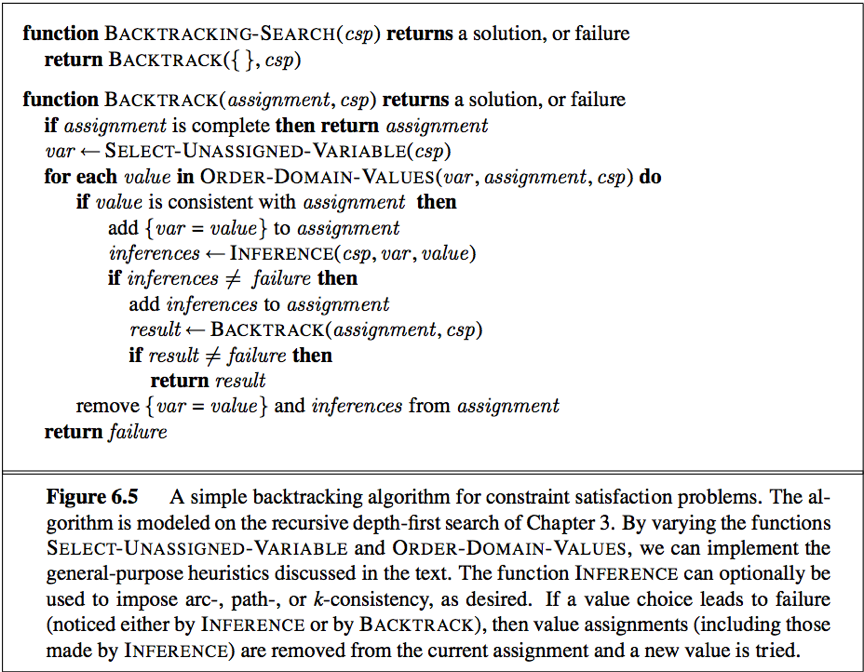
To solve CSPs efficiently without domain-specific knowledge, address following questions:

1)function SELECT-UNASSIGNED-VARIABLE: which variable should be assigned next?

  function ORDER-DOMAIN-VALUES: in what order should its values be tried?

2)function INFERENCE: what inferences should be performed at each step in the search?

3)When the search arrives at an assignment that violates a constraint, can the search avoid repeating this failure?

 

1. Variable and value ordering

 

SELECT-UNASSIGNED-VARIABLE

Variable selection—fail-first

Minimum-remaining-values (MRV) heuristic: The idea of choosing the variable with the fewest “legal” value. A.k.a. “most constrained variable” or “fail-first” heuristic, it picks a variable that is most likely to cause a failure soon thereby pruning the search tree. If some variable X has no legal values left, the MRV heuristic will select X and failure will be detected immediately—avoiding pointless searches through other variables.

E.g. After the assignment for WA=red and NT=green, there is only one possible value for SA, so it makes sense to assign SA=blue next rather than assigning Q.

[Powerful guide]

Degree heuristic: The degree heuristic attempts to reduce the branching factor on future choices by selecting the variable that is involved in the largest number of constraints on other unassigned variables. [useful tie-breaker]

e.g. SA is the variable with highest degree 5; the other variables have degree 2 or 3; T has degree 0.

 

ORDER-DOMAIN-VALUES

Value selection—fail-last

If we are trying to find all the solution to a problem (not just the first one), then the ordering does not matter.

Least-constraining-value heuristic: prefers the value that rules out the fewest choice for the neighboring variables in the constraint graph. (Try to leave the maximum flexibility for subsequent variable assignments.)

e.g. We have generated the partial assignment with WA=red and NT=green and that our next choice is for Q. Blue would be a bad choice because it eliminates the last legal value left for Q’s neighbor, SA, therefore prefers red to blue.

 

The minimum-remaining-values and degree heuristic are domain-independent methods for deciding which variable to choose next in a backtracking search. The least-constraining-value heuristic helps in deciding which value to try first for a given variable.

 

2. Interleaving search and inference

INFERENCE

forward checking: [One of the simplest forms of inference.] Whenever a variable X is assigned, the forward-checking process establishes arc consistency for it: for each unassigned variable Y that is connected to X by a constraint, delete from Y’s domain any value that is inconsistent with the value chosen for X.

There is no reason to do forward checking if we have already done arc consistency as a preprocessing step.

 

Advantage: For many problems the search will be more effective if we combine the MRV heuristic with forward checking.

Disadvantage: Forward checking only makes the current variable arc-consistent, but doesn’t look ahead and make all the other variables arc-consistent.

MAC (Maintaining Arc Consistency) algorithm: [More powerful than forward checking, detect this inconsistency.] After a variable X_i is assigned a value, the INFERENCE procedure calls AC-3, but instead of a queue of all arcs in the CSP, we start with only the arcs(X_j, X_i) for all X_j that are unassigned variables that are neighbors of X_i. From there, AC-3 does constraint propagation in the usual way, and if any variable has its domain reduced to the empty set, the call to AC-3 fails and we know to backtrack immediately.

 

3. Intelligent backtracking

 

chronological backtracking: The BACKGRACKING-SEARCH in Fig 6.5. When a branch of the search fails, back up to the preceding variable and try a different value for it. (The most recent decision point is revisited.)

e.g.

Suppose we have generated the partial assignment {Q=red, NSW=green, V=blue, T=red}.

When we try the next variable SA, we see every value violates a constraint.

We back up to T and try a new color, it cannot resolve the problem.

Intelligent backtracking: Backtrack to a variable that was responsible for making one of the possible values of the next variable (e.g. SA) impossible.

Conflict set for a variable: A set of assignments that are in conflict with some value for that variable.

(e.g. The set {Q=red, NSW=green, V=blue} is the conflict set for SA.)

backjumping method: Backtracks to the most recent assignment in the conflict set.

(e.g. backjumping would jump over T and try a new value for V.)

 

Forward checking can supply the conflict set with no extra work.

Whenever forward checking based on an assignment X=x deletes a value from Y’s domain, add X=x to Y’s conflict set;

If the last value is deleted from Y’s domain, the assignment in the conflict set of Y are added to the conflict set of X.

In fact,every branch pruned by backjumping is also pruned by forward checking. Hence simple backjumping is redundant in a forward-checking search or in a search that uses stronger consistency checking (such as MAC).

 

Conflict-directed backjumping:

e.g.

consider the partial assignment which is proved to be inconsistent: {WA=red, NSW=red}.

We try T=red next and then assign NT, Q, V, SA, no assignment can work for these last 4 variables.

Eventually we run out of value to try at NT, but simple backjumping cannot work because NT doesn’t have a complete conflict set of preceding variables that caused to fail.

The set {WA, NSW} is a deeper notion of the conflict set for NT, caused NT together with any subsequent variables to have no consistent solution. So the algorithm should backtrack to NSW and skip over T.

A backjumping algorithm that uses conflict sets defined in this way is called conflict-direct backjumping.

How to Compute:

When a variable’s domain becomes empty, the “terminal” failure occurs, that variable has a standard conflict set.

Let X_j be the current variable, let conf(X_j) be its conflict set. If every possible value for X_j fails, backjump to the most recent variable X_i in conf(X_j), and set

conf(X_i) ← conf(X_i)∪conf(X_j) – {X_i}.

The conflict set for an variable means, there is no solution from that variable onward, given the preceding assignment to the conflict set.

e.g.

assign WA, NSW, T, NT, Q, V, SA.

SA fails, and its conflict set is {WA, NT, Q}. (standard conflict set)

Backjump to Q, its conflict set is {NT, NSW}∪{WA,NT,Q}-{Q} = {WA, NT, NSW}.

Backtrack to NT, its conflict set is {WA}∪{WA,NT,NSW}-{NT} = {WA, NSW}.

Hence the algorithm backjump to NSW. (over T)

 

After backjumping from a contradiction, how to avoid running into the same problem again:

Constraint learning: The idea of finding a minimum set of variables from the conflict set that causes the problem. This set of variables, along with their corresponding values, is called a no-good. We then record the no-good, either by adding a new constraint to the CSP or by keeping a separate cache of no-goods.

 

Backtracking occurs when no legal assignment can be found for a variable. Conflict-directed backjumping backtracks directly to the source of the problem.

 

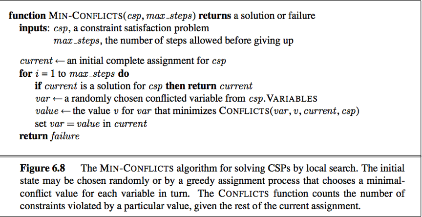
Local search for CSPs

Local search algorithms for CSPs use a complete-state formulation: the initial state assigns a value to every variable, and the search change the value of one variable at a time.

The min-conflicts heuristic: In choosing a new value for a variable, select the value that results in the minimum number of conflicts with other variables.

 

Local search techniques in Section 4.1 can be used in local search for CSPs.

The landscape of a CSP under the mini-conflicts heuristic usually has a series of plateau. Simulated annealing and Plateau search (i.e. allowing sideways moves to another state with the same score) can help local search find its way off the plateau. This wandering on the plateau can be directed with tabu search: keeping a small list of recently visited states and forbidding the algorithm to return to those tates.

 

Constraint weighting: a technique that can help concentrate the search on the important constraints.

Each constraint is given a numeric weight W_i, initially all 1.

At each step, the algorithm chooses a variable/value pair to change that will result in the lowest total weight of all violated constraints.

The weights are then adjusted by incrementing the weight of each constraint that is violated by the current assignment.

 

Local search can be used in an online setting when the problem changes, this is particularly important in scheduling problems.

 

The structure of problem

 

1. The structure of constraint graph

The structure of the problem as represented by the constraint graph can be used to find solution quickly.

e.g. The problem can be decomposed into 2 independent subproblems: Coloring T and coloring the mainland.

 

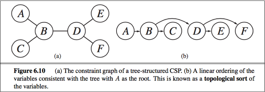
Tree: A constraint graph is a tree when any two varyiable are connected by only one path.

Directed arc consistency (DAC): A CSP is defined to be directed arc-consistent under an ordering of variables X₁, X₂, … , X_n if and only if every X_i is arc-consistent with each X_j for j>i.

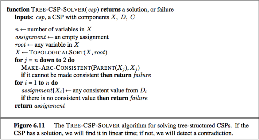
By using DAC, any tree-structured CSP can be solved in time linear in the number of variables.

How to solve a tree-structure CSP:

Pick any variable to be the root of the tree;

Choose an ordering of the variable such that each variable appears after its parent in the tree. (topological sort)

Any tree with n nodes has n-1 arcs, so we can make this graph directed arc-consistent in O(n) steps, each of which must compare up to d possible domain values for 2 variables, for a total time of O(nd²).

Once we have a directed arc-consistent graph, we can just march down the list of variables and choose any remaining value.

Since each link from a parent to its child is arc consistent, we won’t have to backtrack, and can move linearly through the variables.

 

 

There are 2 primary ways to reduce more general constraint graphs to trees:

1. Based on removing nodes;

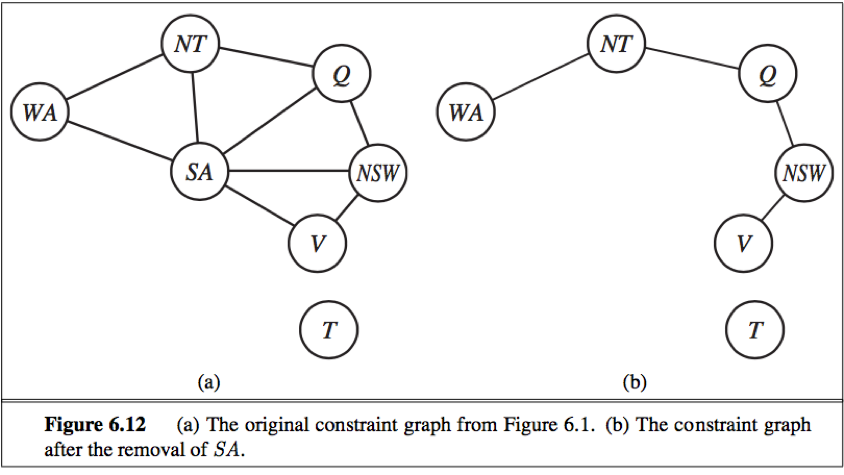
e.g. We can delete SA from the graph by fixing a value for SA and deleting from the domains of other variables any values that are inconsistent with the value chosen for SA.

The general algorithm:

Choose a subset S of the CSP’s variables such that the constraint graph becomes a tree after removal of S. S is called a cycle cutset.

For each possible assignment to the variables in S that satisfies all constraints on S,

  (a) remove from the domain of the remaining variables any values that are inconsistent with the assignment for S, and

  (b) If the remaining CSP has a solution, return it together with the assignment for S.

Time complexity: O(d^c·(n-c)d²), c is the size of the cycle cut set.

Cutset conditioning: The overall algorithmic approach of efficient approximation algorithms to find the smallest cycle cutset.

2. Based on collapsing nodes together

Tree decomposition: construct a tree decomposition of the constraint graph into a set of connected subproblems, each subproblem is solved independently, and the resulting solutions are then combined.

 

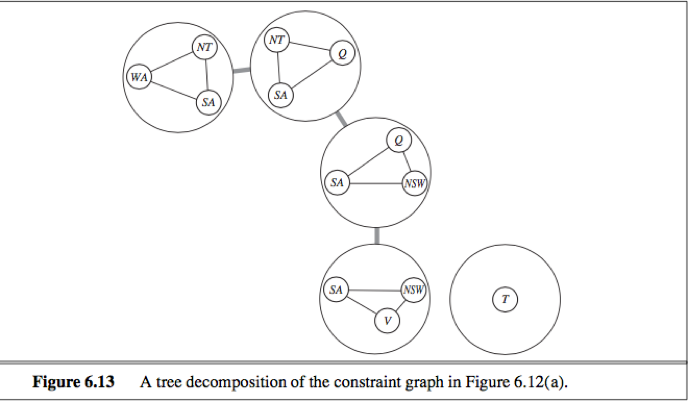
A tree decomposition must satisfy 3 requirements:

·Every variable in the original problem appears in at least one of the subproblems.

·If 2 variables are connected by a constraint in the original problem, they must appear together (along with the constraint) in at least one of the subproblems.

·If a variable appears in 2 subproblems in the tree, it must appear in every subproblem along the path connecting those those subproblems.

 

We solve each subproblem independently.

 If any one has no solution, the entire problem has no solution.

If we can solve all the subproblems, then construct a global solution as follows:

First, view each subproblem as a “mega-variable” whose domain is the set of all solutions for the subproblem.

Then, solve the constraints connecting the subproblems using the efficient algorithm for trees.

 

A given constraint graph admits many tree decomposition;

In choosing a decomposition, the aim is to make the subproblems as small as possible.

Tree width:

The tree width of a tree decomposition of a graph is one less than the size of the largest subproblems.

The tree width of the graph itself is the minimum tree width among all its tree decompositions.

Time complexity: O(nd^w+1), w is the tree width of the graph.

 

The complexity of solving a CSP is strongly related to the structure of its constraint graph. Tree-structured problems can be solved in linear time. Cutset conditioning can reduce a general CSP to a tree-structured one and is quite efficient if a small cutset can be found. Tree decomposition techniques transform the CSP into a tree of subproblems and are efficient if the tree width of constraint graph is small.

 

2. The structure in the values of variables

By introducing a symmetry-breaking constraint, we can break the value symmetry and reduce the search space by a factor of n!.

e.g.

Consider the map-coloring problems with n colors, for every consistent solution, there is actually a set of n! solutions formed by permuting the color names.(value symmetry)

On the Australia map, WA, NT and SA must all have different colors, so there are 3!=6 ways to assign.

We can impose an arbitrary ordering constraint NT<SA<WA that requires the 3 values to be in alphabetical order. This constraint ensures that only one of the n! solution is possible: {NT=blue, SA=green, WA=red}. (symmetry-breaking constraint)

转载于:https://www.cnblogs.com/RDaneelOlivaw/p/8072603.html