


 本文介绍了DGL图的基本属性和成员函数,包括节点特征的限制和图的创建。重点讨论了信息传播的过程,如send和recv函数,以及如何通过prop_nodes进行节点更新。还提到了DGLGraph的常用API,如Computing, Adjacency矩阵和Topology修改。"
111536900,10294821,Electron+Vue实现静默打印小票,"['前端开发', 'Vue', 'Electron', '打印机API']
本文介绍了DGL图的基本属性和成员函数,包括节点特征的限制和图的创建。重点讨论了信息传播的过程,如send和recv函数,以及如何通过prop_nodes进行节点更新。还提到了DGLGraph的常用API,如Computing, Adjacency矩阵和Topology修改。"
111536900,10294821,Electron+Vue实现静默打印小票,"['前端开发', 'Vue', 'Electron', '打印机API']
import torch as th
import dgl
u, v = th.tensor([0,0,0,1]),th.tensor([1,2,3,4])
g = dgl.graph((u,v))#创建图,以元组的方式传入
g输出:Graph(num_nodes=5, num_edges=4,
ndata_schemes={}
edata_schemes={})1.关于图graph的基本属性和成员函数
g.nodes()
tensor([0, 1, 2, 3, 4])
g.edges()
(tensor([0, 0, 0, 1]), tensor([1, 2, 3, 4]))
notes:
如果node id有一个点是孤立点,则需要显示的声明节点个数
eg: g = dgl.graph((u,v),num_nodes = 8)
#创建无向图的2种基本方法:
1.在u和v中声明无向节点:u = [0,1],[1,0],这样就创建了一个0-1之间的无向图
2.用dgl.to_bidirected(g)
关于类型:
#关于类型:节点id支持32or64bit 整型,在创建图的时候,指定idtype = th.int32
#g.long()convert to int 64
#g.int() convert to int 32
#g.idtype查看
节点特征:
通过ndata和edata访问
g = dgl.graph(([0,0,1,5],[1,2,2,0]))
g
Graph(num_nodes=6, num_edges=4,
ndata_schemes={}
edata_schemes={})
g.ndata['x'] = th.ones(g.num_nodes(),3)
g.edata['x'] = th.ones(g.num_edges(),dtype=th.int)
#还可以继续分配其他特征
g.ndata['y'] = th.randn(g.num_nodes(),5)
g.ndata['y'][0]#打印第一个节点y属性值
输出:
tensor([-0.0859, 1.7802, -1.7130, 0.1395, 0.1102])notes:
只接受数值型特征;节点内部的属性名必须不同;节点和边的属性名可以相同 维度必须对应,即节点数必须对应特征的第一维,边数也是如此
其他方式创建图:
#从networkx创建图
import networkx as nx
nx_g = nx.path_graph(5)#无向图
g_net = dgl.from_networkx(nx_g)#dgl默认创建有向图,原本在networkx中是4条边,现在成了8条
g_net
#还可以从文件,像json,csv格式读取图...
输出:
Graph(num_nodes=5, num_edges=8,
ndata_schemes={}
edata_schemes={})创建异质图:
#异质图:在dgl中,二分图也是一种特殊的异质图,源点必须和靶点是绝对的,即一组节点作为源点
#它然后也作为其他源点的靶点,那么这个图的原的src和dgt属性就会发生变化
graph_data = {
('drug','interacts','drug'):(th.tensor([0,1]),th.tensor([1,2])),
('drug','interacts','gene'):(th.tensor([0,1]),th.tensor([2,3])),
('drug','treats','disease'):(th.tensor([1]),th.tensor([2]))
}
g1 = dgl.heterograph(graph_data)
print(g1.srcnodes('drug'))
print(g1.srcnodes('disease'))
print(g1.srcnodes('gene'))
print(g1.dstnodes('drug'))
print(g1.dstnodes('disease'))
print(g1.dstnodes('gene'))#gene其实在源点是没有的,但是因为drug的原因,所有类型的点都既可以作为src,也可以在作为dst
#可以看到靶点和源点是一样的
输出:
tensor([0, 1, 2])
tensor([0, 1, 2])
tensor([0, 1, 2, 3])
tensor([0, 1, 2])
tensor([0, 1, 2])
tensor([0, 1, 2, 3])
#再来看一组:
graph_data = {
('drug','interacts','gene'):(th.tensor([0,1]),th.tensor([2,3])),
('drug','treats','disease'):(th.tensor([1]),th.tensor([2]))
}
g2 = dgl.heterograph(graph_data)
print(g2.srcnodes('drug'))
#print(g2.srcnodes('disease'))
#print(g2.srcnodes('gene'))
#print(g2.dstnodes('drug'))#这3条语句如果存在就会报错
print(g2.dstnodes('disease'))
print(g2.dstnodes('gene'))
输出:
tensor([0, 1])
tensor([0, 1, 2])
tensor([0, 1, 2, 3])
#继续以前面的例子来看,如果是异质图,那么节点类型会有很多种,那么之前提到过的很多种方法都要额外加一个指定类型的值才能访问指定类型节点的一些属性
g1.num_nodes()
g1.num_nodes('drug')
输出:
3
g1.nodes('drug')
输出:
tensor([0, 1, 2])
g1.nodes['drug'].data['hv'] = th.ones(g1.num_nodes('drug'),3)
g1.num_edges('treats')
输出:
1
#对于边:比较特殊,看下面的一段话:
"""
When the edge type uniquely determines the types of source and destination nodes,
one can just use one string instead of a string triplet to specify the edge type.
For example, for a heterograph with two relations ('user', 'plays', 'game') and ('user', 'likes', 'game'),
it is safe to just use 'plays' or 'likes' to refer to the two relations.
"""
#interacts对应的是2条边,如果仅用interacts,则会模糊不知道是哪个类型
#g1.num_edges('interacts')#会报错
g1.edges[('drug','interacts','gene')]#必须以三元组方式传入
输出:
EdgeSpace(data={})
g1.num_edges(('drug','interacts','drug'))
输出: 2
g1.num_edges(('drug','interacts','gene'))
输出:2
CPU与GPU交互:
#CPU与GPU交互,dgl的图有一个device属性,可以查看当前图所在的设备
#g.device
#g.ndata['x'].data
#to('cuda:0')
二、信息传播和一些graph的成员函数
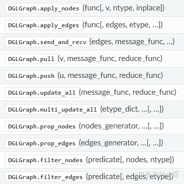
信息传播,信息传播说白了就是一个映射(操作),相对于torch,就是普通的sum,mean,conv函数,在此基础上将其组合封装,就得到了layer,这是针对于图数据的layer,对应于torch的layer;
其次,针对于图数据,她是如何做的呢?因为图有节点和边,它可以沿着边发射信息(send),然后对应的节点接受信息 (receive),所以dgl也是有这2个函数的,但是后来为了节省内存,很多函数都在内部封装了这一过程(结合了send和recv),
原因: 分开的时候,要存储中间的临时信息,需要占用内存,当图很大时,很容易不够用,然后官方是这么说的,直接把这2者结合,线程啥的,就不会 用那么多内存了。 send(edges, message_func) for computing the messages along the given edges.沿着给定边发送信息,这个信息可以是对节点的邻居做sum,mean,函数返回的结果应该是每个节点都多了一个发送过来的信息组成的属性
#用户自定义:
G.update_all(lambda edges: {'m' : edges.src['h']},
             lambda nodes: {'h' : sum(nodes.mailbox['m'], axis=1)})
#built-in:
G.update_all(fn.copy_src('h', 'm'), fn.sum('m', 'h'))
我特地去简单看了一下源码,好吧,我放弃了 recv(nodes, reduce_func) for collecting the incoming messages, perform aggregation and so on.基于发送的信息,对该信息进行处理,为啥叫reduce呢 因为会涉及到多个邻居时的降维,从而保持列维度的一致性。
Although the two-stage abstraction can cover all the models that are defined in the message passing paradigm, it is inefficient because it requires storing explicit messages. See the DGL blog post for more details and performance results.
官网的一段话:
Our solution, also explained in the blog post, is to fuse the two stages into one kernel so no explicit messages are generated and stored
https://www.dgl.ai/blog/2019/05/04/kernel.htmlwww.dgl.ai(官网)
prop_nodes:
import dgl.function as fn
g = dgl.heterograph({('user', 'follows', 'user'): ([0, 1, 2, 3], [2, 3, 4, 4])})
g.nodes['user'].data['h'] = th.tensor([[1.], [2.], [3.], [4.], [5.]])
g['follows'].prop_nodes([[0,1,2,3],[4]], fn.copy_src('h', 'm'),
fn.sum('m', 'h'), etype='follows')
g.nodes['user'].data['h']
输出:
tensor([[0.],
[0.],
[1.],
[2.],
[3.]])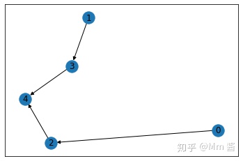
The nodes in the same frontier will be triggered together, while nodes in different frontiers will be triggered according to the generating order. node_generator中每个元素都是frontier,每个frontier中,将会一起pull,后面的frontier将会在前面的基础上进行迭代(按照迭代顺序迭代);在以上的例子中,先以节点[0,1,2,3]开始迭代,每个节点上运用pull函数:
0->0(因为0没有源节点)
1->0(同上)
2->1(因为2的源节点是0,0对应的数值是1,在这一轮之前0还未发生变化)
3->2
第一轮结束,节点的值进行更新
从[4]开始迭代:
4的源节点是3和2,所以
5->3(因为2和3节点的值分别对应1和2)
最终结果:0,0,1,2,3
深度优先遍历:
g = dgl.graph([(0, 1), (1, 2), (1, 3), (2, 4), (2, 5),(3,6),(3,7),(7,8)])
list(dgl.bfs_edges_generator(g, 0))
#广度优先遍历,给定起始点,开始访问邻居节点,被访问过不再访问,如果有多个邻居,则优先访问ID较小的,直到最后没有
#邻居节点,返回由边id组成的列表,每个元素都是当前结点的邻边id集合
输出:
[tensor([0]), tensor([1, 2]), tensor([3, 4, 5, 6]), tensor([7])]
有点类似与层次遍历:
边0
边1,2(节点id小的先访问)
边3,4,5,6
边7

list(dgl.dfs_edges_generator(g, 0))
#深度,给定起始点,沿着边一直访问,直到最后没有邻居节点,返回由边id组成的列表,每个元素都是当前节点的一个边(就一个)
#如果还有边,则退回到最后访问,直到访问完。
输出:
[tensor([0]),
 tensor([1]),
 tensor([3]),
 tensor([4]),
 tensor([2]),
 tensor([5]),
 tensor([6]),
 tensor([7])]
这本质上是一个二叉树的先序遍历,
边0->1->3
边4
边2->5
边6->7

可视化:上面的实际上是一个二叉树,因为用networkx画图,画出来的很乱,所以就用其他软件了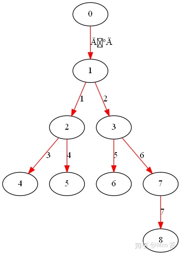
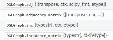
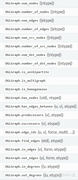
附:常用的dgl.graph还有以下一些API:
Computing with DGLGraph
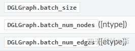
Querying batch summary
Mutating topology
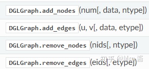
Adjacency and incidence matrix
Querying graph structure
后面还会继续记录Message prop,dataloader,dgl.nn,以及整个的几种典型的pipline


 7429
7429

 被折叠的 条评论
为什么被折叠?
被折叠的 条评论
为什么被折叠?
 到【灌水乐园】发言


