Machine Learning for Developers

Machine Learning for Developers

Most developers these days have heard of machine learning, but when trying to find an 'easy' way into this technique, most people find themselves getting scared off by the abstractness of the concept of Machine Learning and terms asregression, unsupervised learning, Probability Density Function and many other definitions. If one switches to books there are books such as An Introduction to Statistical Learning with Applications in R and Machine Learning for Hackers who use programming language R for their examples.

However R is not really a programming language in which one writes programs for everyday use such as is done with for example Java, C#, Scala etc. This is why in this blog machine learning will be introduced using Smile, a machine learning library that can be used both in Java and Scala. These are languages that most developers have seen at least once during their study or career.

The first section 'The global idea of machine learning' contains all important concepts and notions you need to know about to get started with the practical examples that are described in the section 'Practical Examples'. The section practical examples is inspired by the examples from the book Machine Learning for Hackers. Additionally the book Machine Learning in Action was used for validation purposes.

The second section Practical examples contains examples for various machine learning (ML) applications, with Smile as ML library.

Note that in this blog, 'new' definitions are hyperlinked such that if you want, you can read more regarding that specific topic, but you are not obliged to do this in order to be able to work through the examples.

As final note I'd like to thank the following people:

• Haifeng Li for his support and writing the awesome and free to use library Smile.
• Erik Meijer for all suggestions and supervision of the process of writing this blog.
• Richard van Heest for his feedback and co-reading the blog.
• Lars Willems for his feedback and co-reading the blog.

 The global idea of machine learning

You probably have heard about Machine learning as a concept one time or another. However, if you would have to explain what machine learning is to another person, how would you do this? Think about this for a second before reading the rest of this section.

Machine learning is explained in many ways, some more accurate than others, however there is a lot of inconsistency in its definition. Some say machine learning is generating a static model based on historical data, which then allows you to predict for future data. Others say it's a dynamic model that keeps on changing as more data is added over time.

I agree more with the dynamic definition but due to certain limitations we explain the static model method in the examples. However, we do explain how the dynamic principle would work in the subsection Dynamic machine learning.

The upcoming subsections explain commonly used definitions and notions in the machine learning field. We advise you to read through these before starting the practical examples.

 Features

A feature is a property on which a model is trained. Say for example that you classify emails as spam/ham based on the frequency of the word 'Buy' and 'Money'. Then these words are features, or part of a feature if you would combine it with more words. If you would use machine learning to predict whether one is a friend of yours, the amount of 'common' friends could be a feature. Note that in the field, sometimes features are also referred to as attributes.

 Model

When one talks about machine learning, often the term model is mentioned. The model is the result of any machine learning method and the algorithm used within this method. This model can be used to make predictions in supervised, or to retrieve clusterings in unsupervised learning. Chances are high that you will encounter the terms online and offlinetraining of a model in the field. The idea behind online training is that you add training data to an already existing model, whereas with offline training you generate a new model from scratch. For performance reasons, online training would be the most preferable method. However for some algorithms this is not possible.

 Learning methods

In the field of machine learning there are two leading ways of learning, namely Supervised learning and Unsupervised learning. A brief introduction is necessary when you want to use Machine learning in your applications, as picking the right machine learning approach and algorithm is an important but sometimes also a little tedious process.

 Supervised learning

In supervised learning you define explicitly what features you want to use, and what output you expect. An example is predicting gender based on height and weight, which is known as a Classification problem. Additionally you can also predict absolute values with Regression. An example of regression with the same data would be predicting one's length based on gender and weight. Some supervised algorithms can only be used for either classification or regression, such asK-NN. However there also exists algorithms such as Support Vector Machines which can be used for both purposes.

 Classification

The problem of classification within the domain of Supervised learning is relatively simple. Given a set of labels, and some data that already received the correct labels, we want to be able to predict labels for new data that we did not label yet. However, before thinking of your data as a classification problem, you should look at what the data looks like. If there is a clear structure in the data such that you can easily draw a regression line it might be better to use a regression algorithm instead. Given the data does not fit to a regression line, or when performance becomes an issue, classification is a good alternative.

An example of a classification problem would be to classify emails as ham or spam based on their content. Given a training set in which emails are labeled ham or spam, a classification algorithm can be used to train a Model. This model can then be used to predict for future emails whether they are ham or spam. A typical example of a classification algorithm is the K-NN algorithm. Another commonly used example of a classification problem is Classifying email as spam or hamwhich is also one of the examples written on this blog.

 Regression

Regression is a lot stronger in comparison to classification. This is because in regression you are predicting actual values, rather than labels. Let us clarify this with a short example: given a table of weights, heights, and genders, you can use K-NN to predict one's gender when given a weight and height. With this same dataset using regression, you could instead predict one's weight or height, given the gender and the respective other missing parameter.

With this extra power, comes great responsibility, thus in the working field of regression one should be very careful when generating the model. Common pitfalls are overfitting, underfitting and not taking into account how the model handlesextrapolation and interpolation.

 Unsupervised learning

In contrast to supervised, with unsupervised learning you do not exactly know the output on beforehand. The idea when applying unsupervised learning is to find hidden underlying structure in a dataset. An example would be PCA with which you can reduce the amount of features by combining features. This combining is done based on the possibly hidden correlation between these features. Another example of unsupervised learning is K-means clustering. The idea behind K-means clustering is to find groups within a dataset, such that these groups can later on be used for purposes such assupervised learning.

 Principal Components Analysis (PCA)

Principal Components Analysis is a technique used in statistics to convert a set of correlated columns into a smaller set of uncorrelated columns, reducing the amount of features of a problem. This smaller set of columns are called the principal components. This technique is mostly used in exploratory data analysis as it reveals internal structure in the data that can not be found with eye-balling the data.

A big weakness of PCA however are outliers in the data. These heavily influence its result, thus looking at the data on beforehand, eliminating large outliers can greatly improve its performance.

To give a clear idea of what PCA does, we show the plots of a dataset of points with 2 dimensions in comparison to the same dataset plotted after PCA is applied.

 

On the left plot the original data is shown, where each color represents a different class. It is clear that from the 2 dimensions (X and Y) you could reduce to 1 dimension and still classify properly. This is where PCA comes in place. With PCA a new value is calculated for each datapoint, based on its original dimensions.

In the plot on the right you see the result of applying PCA to this data. Note that there is a y value, but this is purely to be able to plot the data and show it to you. This Y value is 0 for all values as only the X values are returned by the PCA algorithm. Also note that the values for X in the right plot do not correspond to the values in the left plot, this shows that PCA not 'just drops' a dimension.

 Validation techniques

In this section we will explain some of the techniques available for model validation, and some terms that are commonly used in the Machine Learning field within the scope of validation techniques.

 Cross validation

The technique of cross validation is one of the most common techniques in the field of machine learning. Its essence is toignore part of your dataset while training your model, and then using the model to predict this ignored data. Comparing the predictions to the actual value then gives an indication of the performance of your model, and the quality of your training data.

The most important part of this cross validation is the splitting of data. You should always use the complete dataset when performing this technique. In other words you should not randomly select X datapoints for training and then randomly select X datapoints for testing, because then some datapoints can be in both sets while others might not be used at all.

 (2 fold) Cross validation

In 2-fold cross validation you perform a split of the data into test and training for each fold (so 2 times) and train a model using the training dataset, followed by verification with the testing set. Doing so allows you to compute the error in the predictions for the test data 2 times. These error values then should not differ significantly. If they do, either something is wrong with your data or with the features you selected for model prediction. Either way you should look into the data more and find out what is happening for your specific case, as training a model based on the data might result in an overfittedmodel for erroneous data.

 Regularization

The basic idea of regularization is preventing overfitting your model by simplifying it. Suppose your data is a 3rd degree polynomial function, but your data has noise and this would cause the model to be of a higher degree. Then the model would perform poorly on new data, whereas it seems to be a good model at first. Regularization helps preventing this, by simplifying the model with a certain value lambda. However to find the right lambda for a model is hard when you have no idea as to when the model is overfitted or not. This is why cross validation is often used to find the best lambda fitting your model.

 Precision

In the field of computer science we use the term precision to define the amount of items selected which are actually relevant. So when you compute the precision value for a search algorithm on documents, the precision of that algorithm is defined by how many documents from the result set are actually relevant.

This value is computed as follows:

As this might be a bit hard to grasp I will give an example:

Say we have documents {aa, ab, bc, bd, ee} as the complete corpus, and we query for documents with a in the name. If our algorithm would then return the document set {aa, ab}, the precision would be 100% intuitively. Let's verify it by filling in the formula:

Indeed it is 100%. If we would run the query again but get more results than only {aa, ab}, say we additionally get {bc,de} back as well, this influences the precision as follows:

Here the results contained the relevant results but also 2 irrelevant results. This caused the precision to decrease. However if you would calculate the recall for this example it would be 100%. This is how precision and recall differ from each other.

 Recall

Recall is used to define the amount of relevant items that are retrieved by an algorithm given a query and a data corpus. So given a set of documents, and a query that should return a subset of those documents, the recall value represents how many of the relevant documents are actually returned. This value is computed as follows:

Given this formula, let's do an example to see how it works:

Say we have documents {aa,ab,bc,bd,ee} as complete corpus and we query for documents with a in the name. If our algorithm would be to return {aa,ab} the recall would be 100% intuitively. Let's verify it by filling in the formula:

Indeed it is 100%. Next we shall show what happens if not all relevant results are returned:

Here the results only contained half of the relevant results. This caused the recall to decrease. However if you would compute the precision for this situation, it would result in 100% precision, because all results are relevant.

 Prior

The prior value that belongs to a classifier given a datapoint represents the likelihood that this datapoint belongs to this classifier. In practice this means that when you get a prediction for a datapoint, the prior value that is given with it, represents how 'convinced' the model is regarding the classification given to that datapoint.

 Root Mean Squared Error (RMSE)

The Root Mean Squared Error (RMSE or RMSD where D stands for deviation) is the square root of the mean of the squared differences between the actual value and predicted value. As this is might be hard to grasp, I'll explain it using an example. Suppose we have the following values:

Predicted temperature	Actual temperature	squared difference for Model	square difference for average
10	12	4	7.1111
20	17	9	5.4444
15	15	0	0.1111

The mean of these squared differences for the model is 4.33333, and the root of this is 2.081666. So in average, the model predicts the values with an error of 2.08. The lower this RMSE value is, the better the model is in its predictions. This is why in the field, when selecting features, one computes the RMSE with and without a certain feature, in order to say something about how that feature affects the performance of the model. With this information one can then decide whether the additional computation time for this feature is worth it in comparison to the improvement rate on the model.

Additionally, because the RMSE is an absolute value, it can be normalised in order to compare models. This results in the Normalised Root Mean Square Error (NRMSE). For computing this however, you need to know the minimum and maximum value that the system can contain. Let's suppose we can have temperatures ranging from minimum of 5 to a maximum of 25 degrees, then computing the NRMSE is as follows:

When we fill in the actual values we get the following result:

Now what is this 10.45 value? This is the error percentage the model has in average on its datapoints.

Finally we can use RMSE to compute a value that is known in the field as R Squared. This value represents how good the model performs in comparison to ignoring the model and just taking the average for each value. For that you need to calculate the RMSE for the average first. This is 4.22222 (taking the mean of the values from the last column in the table), and the root is then 2.054805. The first thing you should notice is that this value is lower than that of the model. This is not a good sign, because this means the model performs worse than just taking the mean. However to demonstrate how to compute R Squared we will continue the computations.

We now have the RMSE for both the model and the mean, and then computing how well the model performs in comparison to the mean is done as follows:

This results in the following computation:

Now what does this -1.307229 represent? Basically it says that the model that predicted these values performs about 1.31 percent worse than returning the average each time a value is to be predicted. In other words, we could better use the average function as a predictor rather than the model in this specific case.

 Common pitfalls

This section describes some common pitfalls in applying machine learning techniques. The idea of this section is to make you aware of these pitfalls and help you prevent actually walking into one yourself.

 Overfitting

When fitting a function on the data, there is a possibility the data contains noise (for example by measurement errors). If you fit every point from the data exactly, you incorporate this noise into the model. This causes the model to predict really well on your test data, but relatively poor on future data.

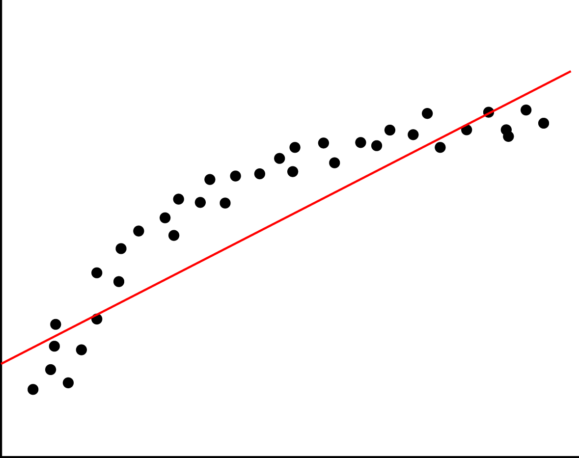
The left image here below shows how this overfitting would look like if you were to plot your data and the fitted functions, whereas the right image would represent a good fit of the regression line through the datapoints.

 

Overfitting can easily happen when applying regression but can just as easily be introduced in Naive Bayes classifications. In regression it happens with rounding, bad measurements and noisy data. In naive bayes however, it could be the features that were picked. An example for this would be classifying spam or ham while keeping all stop words.

Overfitting can be detected by performing validation techniques and looking into your data's statistical features, and detecting and removing outliers.

 Underfitting

When you are turning your data into a model, but are leaving (a lot of) statistical data behind, this is called underfitting. This can happen due to various reasons, such as using a wrong regression type on the data. If you have a non-linear structure in the data, and you apply linear regression, this would result in an under-fitted model. The left image here below represents an under-fitted regression line whereas the right image shows a good fit regression line.

 

You can prevent underfitting by plotting the data to get insights in the underlying structure, and using validation techniquessuch as cross validation.

 Curse of dimensionality

The curse of dimensionality is a collection of problems that can occur when your data size is lower than the amount of features (dimensions) you are trying to use to create your machine learning model. An example of a dimensionality curse is matrix rank deficiency. When using Ordinary Least Squares(OLS), the underlying algorithm solves a linear system in order to build up a model. However if you have more columns than you have rows, coming up with a single solution for this system is not possible. If this is the case, the best solution would be to get more datapoints or reduce the feature set.

If you want to know more regarding this curse of dimensionality, there is a study focussed on this issue. In this study, researchers Haifeng Li, Keshu Zhang and Tao Jiang developed an algorithm that improves cancer classification with very few datapoints. They compared their algorithm with support vector machines and random forests.

 Dynamic machine learning

In almost all literature you can find about machine learning, a static model is generated and validated, and then used for predictions or recommendations. However in practice, this alone would not make a very good machine learning application. This is why in this section we will explain how to turn a static model into a dynamic model. Since the (most optimal) implementation depends on the algorithm you are using, we will explain the concept rather than giving a practical example. Because explaining it in text only will not be very clear we first present you the whole system in a diagram. We will then use this diagram to explain machine learning and how to make the system dynamic.

The basic idea of machine learning can be described by the following steps:

1. Gather data
2. Split the data into a testing and training set
3. Train a model (with help of a machine learning algorithm)
4. Validate the model with a validation method which takes the model and testing data
5. do predictions based on the model

In this process there are a few steps missing when it comes to actual applications in the field. These steps are in my opinion the most important steps to make a system actually learn.

The idea behind what we call dynamic machine learning is as follows: You take your predictions, combine it with user feedback and feed it back into your system to improve your dataset and model. As we just said we need user feedback, so how is this gained? Let's take friend suggestions on Facebook for example. The user is presented 2 options: 'Add Friend' or 'Remove'. Based on the decision of the user, you have direct feedback regarding that prediction.

So say you have this user feedback, then you can apply machine learning over your machine learning application to learn about the feedback that is given. This might sound a bit strange, but we will try to explain this more elaborately. However before we do this, we need to make a disclaimer: our description of the Facebook friend suggestion system is a 100% assumption and in no way confirmed by Facebook itself. Their systems are a secret to the outside world as far as we know.

Say the system predicts based on the following features:

1. amount of common friends
2. Same hometown
3. Same age

Then you can compute a prior for every person on Facebook regarding the chance that he/she is a good suggestion to be your friend. Say you store the results of all these predictions for a period of time, then analysing this data on its own with machine learning allows you to improve your system. To elaborate on this, say most of our 'removed' suggestions had a high rating on feature 2, but relatively low on 1, then we can add weights to the prediction system such that feature 1 is more important than feature 2. This will then improve the recommendation system for us.

Additionally, the dataset grows over time, so we should keep on updating our model with the new data to make the predictions more accurate. How to do this however, depends on the size and mutation rate of your data.

 Practical examples

In this section we present you a set of machine learning algorithms in a practical setting. The idea of these examples is to get you started with machine learning algorithms without an in depth explanation of the underlying algorithms. We focus purely on the functional aspect of these algorithms, how you can verify your implementation and finally try to make you aware of common pitfalls.

The following examples are available:

• Labeling ISP's based on their down/upload speed (K-NN)
• Classifying email as spam or ham (Naive Bayes)
• Ranking emails based on their content (Recommendation system)
• Predicting weight based on height (Linear Regression OLS)
• An attempt at rank prediction for top selling books using text regression
• Using unsupervised learning to merge features (PCA)
• Using Support Vector Machines (SVMS)

For each of these examples we used the Smile Machine Learning library. We used both the smile-core and smile-plot libraries. These libraries are available on Maven, Gradle, Ivy, SBT and Leiningen. Information on how to add them using one of these systems can be found here for the core, and here for the plotting library.

So before you start working through an example, I assume you made a new project in your favourite IDE, and added thesmile-core and smile-plot libraries to your project. Additional libraries when used, and how to get the example data is addressed per example.

 Labeling ISPs based on their down/upload speed (K-NN using Smile in Scala)

The goal of this section is to use the K-Nearest Neighbours (K-NN) Algorithm to classify download/upload speed pairs asinternet service provider (ISP) Alpha (represented by 0) or Beta (represented by 1). The idea behind K-NN is as follows: given a set of points that are classified, you can classify the new point by looking at its K neighbours (K being a positive integer). The idea is that you find the K-neighbours by looking at the euclidean distance between the new point and its surrounding points. For these neighbours you then look at the biggest representative class and assign that class to the new point.

To start this example you should download the example data. Additionally you should set the path in the code snippet to where you stored this example data.

The first step is to load the CSV data file. As this is no rocket science, I provide the code for this without further explanation:

object KNNExample {
   def main(args: Array[String]): Unit = { val basePath = "/.../KNN_Example_1.csv" val testData = getDataFromCSV(new File(basePath)) } def getDataFromCSV(file: File): (Array[Array[Double]], Array[Int]) = { val source = scala.io.Source.fromFile(file) val data = source .getLines() .drop(1) .map(x => getDataFromString(x)) .toArray source.close() val dataPoints = data.map(x => x._1) val classifierArray = data.map(x => x._2) return (dataPoints, classifierArray) } def getDataFromString(dataString: String): (Array[Double], Int) = { //Split the comma separated value string into an array of strings val dataArray: Array[String] = dataString.split(',') //Extract the values from the strings val xCoordinate: Double = dataArray(0).toDouble val yCoordinate: Double = dataArray(1).toDouble val classifier: Int = dataArray(2).toInt //And return the result in a format that can later //easily be used to feed to Smile return (Array(xCoordinate, yCoordinate), classifier) } }

First thing you might wonder now is why is the data formatted this way. Well, the separation between dataPoints and their label values is for easy splitting between testing and training data, and because the API expects the data this way for both executing the K-NN algorithm and plotting the data. Secondly the datapoints stored as an Array[Array[Double]] is done to support datapoints in more than just 2 dimensions.

Given the data the first thing to do next is to see what the data looks like. For this Smile provides a nice plotting library. In order to use this however, the application should be changed to a Swing application. Additionally the data should be fed to the plotting library to get a JPane with the actual plot. After changing your code it should look like this:

 object KNNExample extends SimpleSwingApplication {
  def top = new MainFrame { title = "KNN Example" val basePath = "/.../KNN_Example_1.csv" val testData = getDataFromCSV(new File(basePath)) val plot = ScatterPlot.plot(testData._1, testData._2, '@', Array(Color.red, Color.blue) ) peer.setContentPane(plot) size = new Dimension(400, 400) } ...

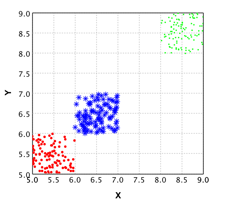
The idea behind plotting the data is to verify whether K-NN is a fitting Machine Learning algorithm for this specific set of data. In this case the data looks as follows:

In this plot you can see that the blue and red points seem to be mixed in the area (3 < x < 5) and (5 < y < 7.5). Since the groups are mixed the K-NN algorithm is a good choice, as fitting a linear decision boundary would cause a lot of false classifications in the mixed area.

Given this choice to use the K-NN algorithm to be a good fit for this problem, let's continue with the actual Machine Learning part. For this the GUI is ditched since it does not really add any value. Recall from the section The global idea of Machine Learning that in machine learning there are 2 key parts: Prediction and Validation. First we will look at the validation, as using a model without any validation is never a good idea. The main reason to validate the model here is to prevent overfitting. However, before we even can do validation, a correct K should be chosen.

The drawback is that there is no golden rule for finding the correct K. However, finding a good K that allows for most datapoints to be classified correctly can be done by looking at the data. Additionally the K should be picked carefully to prevent undecidability by the algorithm. Say for example K=2, and the problem has 2 labels, then when a point is between both labels, which one should the algorithm pick. There is a rule of thumb that K should be the square root of the number of features (on other words the number of dimensions). In our example this would be K=1, but this is not really a good idea since this would lead to higher false-classifications around decision boundaries. Picking K=2 would result in the error regarding our two labels, thus picking K=3 seems like a good fit for now.

For this example we do 2-fold Cross Validation. In general 2-fold cross validation is a rather weak method of model Validation, as it splits the dataset in half and only validates twice, which still allows for overfitting, but since the dataset is only 100 points, 10-fold (which is a stronger version) does not make sense, since then there would only be 10 datapoints used for testing, which would give a skewed error rate.

  def main(args: Array[String]): Unit = { val basePath = "/.../KNN_Example_1.csv" val testData = getDataFromCSV(new File(basePath)) //Define the amount of rounds, in our case 2 and //initialise the cross validation val cv = new CrossValidation(testData._2.length, validationRounds) val testDataWithIndices = (testData ._1 .zipWithIndex, testData ._2 .zipWithIndex) val trainingDPSets = cv.train .map(indexList => indexList .map(index => testDataWithIndices ._1.collectFirst { case (dp, `index`) => dp}.get)) val trainingClassifierSets = cv.train .map(indexList => indexList .map(index => testDataWithIndices ._2.collectFirst { case (dp, `index`) => dp}.get)) val testingDPSets = cv.test .map(indexList => indexList .map(index => testDataWithIndices ._1.collectFirst { case (dp, `index`) => dp}.get)) val testingClassifierSets = cv.test .map(indexList => indexList .map(index => testDataWithIndices ._2.collectFirst { case (dp, `index`) => dp}.get)) val validationRoundRecords = trainingDPSets .zipWithIndex.map(x => ( x._1, trainingClassifierSets(x._2), testingDPSets(x._2), testingClassifierSets(x._2) ) ) validationRoundRecords .foreach { record => val knn = KNN.learn(testData._1, testData._2, 3) //And for each test data point make a prediction with the model val predictions = record ._3 .map(x => knn.predict(x)) .zipWithIndex //Finally evaluate the predictions as correct or incorrect //and count the amount of wrongly classified data points. val error = predictions .map(x => if (x._1 != record._4(x._2)) 1 else 0) .sum println("False prediction rate: " + error / predictions.length * 100 + "%") } }

If you execute this code several times you might notice the false prediction rate to fluctuate quite a bit. This is due to the random samples taken for training and testing. When this random sample is taken a bit unfortunate, the error rate becomes much higher while when taking a good random sample, the error rate could be extremely low.

Unfortunately I cannot provide you with a golden rule to when your model was trained with the best possible training set. One would say that the model with the least error rate is always the best, but when you recall the term overfitting, picking this particular model might perform really bad on future data. This is why having a large enough and representative dataset is key to a good Machine Learning application. However, when aware of this issue, you could implement manners to keep updating your model based on new data and known correct classifications.

Let's recap what we've done so far. First you took care of getting the training and testing data. Next up you generated and validated several models and picked the model which gave the best results. Then we now have one final step to do, which is making predictions using this model:

val knn = KNN.learn(record._1, record._2, 3)
val unknownDataPoint = Array(5.3, 4.3) val result = knn.predict(unknownDatapoint) if (result == 0) { println("Internet Service Provider Alpha") } else if (result == 1) { println("Internet Service Provider Beta") } else { println("Unexpected prediction") } 

The result of executing this code is labeling the unknownDataPoint (5.3, 4.3) as ISP Alpha. This is one of the easier points to classify as it is clearly in the Alpha field of the datapoints in the plot. As it is now clear how to do these predictions I won't present you with other points, but feel free to try out how different points get predicted.

 Classifying email as spam or ham (Naive Bayes)

In this example we will be using the Naive Bayes algorithm to classify email as ham (good emails) or spam (bad emails) based on their content. The Naive Bayes algorithm calculates the probability for an object for each possible class, and then returns the class with the highest probability. For this probability calculation the algorithm uses features. The reason it's called Naive Bayes is because it does not incorporate any correlation between features. In other words, each feature counts the same. I'll explain a bit more using an example:

Say you are classifying fruits and vegetables based on the features color, diameter and shape and you have the following classes: apple, tomato, and cranberry.

Suppose you then want to classify an object with the following values for the features: (red,4 cm, round). This would obviously be a tomato for us, as it is way to small to be an apple, and too large for a cranberry. However, because the Naive Bayes algorithm evaluates each feature individually it will classify it as follows:

• Apple 66.6% probable (based on color, and shape)
• Tomato 100.0% probable (based on color, shape and size)
• cranberry 66.6% probable (based on color and shape)

Thus even though it seems really obvious that it can't be a cranberry or apple, Naive Bayes still gives it a 66.6% change of being either one. So even though it classifies the tomato correctly, it can give poor results in edge cases where the size is just outside the scope of the training set. However, for spam classification Naive Bayes works well, as spam or ham cannot be classified purely based on one feature (word).

As you should now have an idea on how the Naive Bayes algorithm works, we can continue with the actual example. For this example we will use the Naive Bayes implementation from Smile in Scala to classify emails as spam or ham based on their content.

Before we can start however, you should download the data for this example from the SpamAssasins public corpus. The data you need for the example is the easy_ham and spam files, but the rest can also be used in case you feel like experimenting some more. You should unzip these files and adjust the file paths in the code snippets to match the location of the folders. Additionally you will need the stop words file for filtering purposes.

As with every machine learning implementation, the first step is to load in the training data. However in this example we are taking it 1 step further into machine learning. In the KNN examples we had the download and upload speed as features. We did not refer to them as features, as they were the only properties available. For spam classification it is not completely trivial what to use as features. One can use the Sender, the subject, the message content, and even the time of sending as features for classifying as spam or ham.

In this example we will use the content of the email as feature. By this we mean we will select the features (words in this case) from the bodies of the emails in the training set. In order to be able to do this, we need to build a Term Document Matrix (TDM).

We will start off with writing the functions for loading the example data. This will be done with a getMessage method which gets a filtered body from an email given a File as parameter.

def getMessage(file : File)  : String = { //Note that the encoding of the example files is latin1, // thus this should be passed to the fromFile method. val source = scala.io.Source.fromFile(file)("latin1") val lines = source.getLines mkString "\n" source.close() //Find the first line break in the email, //as this indicates the message body val firstLineBreak = lines.indexOf("\n\n") //Return the message body filtered by only text from a-z and to lower case return lines .substring(firstLineBreak) .replace("\n"," ") .replaceAll("[^a-zA-Z ]","") .toLowerCase() }

Now we need a method that gets all the filenames for the emails, from the example data folder structure that we provided you with.

  def getFilesFromDir(path: String):List[File] = { val d = new File(path) if (d.exists && d.isDirectory) { //Remove the mac os basic storage file, //and alternatively for unix systems "cmds" d .listFiles .filter(x => x .isFile && !x .toString .contains(".DS_Store") && !x .toString .contains("cmds")) .toList } else { List[File]() } }

And finally let's define a set of paths that make it easier to load the different datasets from the example data. Together with this we also directly define a sample size of 500, as this is the complete amount of training emails available for the spam set. We take the same amount of ham emails as the training set should be balanced for these two classification groups.

  def main(args: Array[String]): Unit = { val basePath = "/Users/../Downloads/data" val spamPath = basePath + "/spam" val spam2Path = basePath + "/spam_2" val easyHamPath = basePath + "/easy_ham" val easyHam2Path = basePath + "/easy_ham_2" val amountOfSamplesPerSet = 500 val amountOfFeaturesToTake = 100 //First get a subset of the filenames for the spam // sample set (500 is the complete set in this case) val listOfSpamFiles = getFilesFromDir(spamPath) .take(amountOfSamplesPerSet) //Then get the messages that are contained in these files val spamMails = listOfSpamFiles.map(x => (x, getMessage(x))) //Get a subset of the filenames from the ham sample set // (note that in this case it is not necessary to randomly // sample as the emails are already randomly ordered) val listOfHamFiles = getFilesFromDir(easyHamPath) .take(amountOfSamplesPerSet) //Get the messages that are contained in the ham files val hamMails = listOfHamFiles .map{x => (x,getMessage(x)) } } 

Now that we have the training data for both the ham and the spam email, we can start building 2 TDM's. But before we show you the code for this, let's first explain shortly why we actually need this. The TDM will contain ALL words which are contained in the bodies of the training set, including frequency rate. However, since frequency might not be the best measure (as 1 email which contains 1.000.000 times the word 'cake' would mess up the complete table) we will also compute the occurrence rate. By this we mean, the amount of documents that contain that specific term. So let's start off with generating the two TDM's.

 val spamTDM  = spamMails
      .flatMap(email => email
        ._2.split(" ") .filter(word => word.nonEmpty) .map(word => (email._1.getName,word))) .groupBy(x => x._2) .map(x => (x._1, x._2.groupBy(x => x._1))) .map(x => (x._1, x._2.map( y => (y._1, y._2.length)))) .toList //Sort the words by occurrence rate descending //(amount of times the word occurs among all documents) val sortedSpamTDM = spamTDM .sortBy(x => - (x._2.size.toDouble / spamMails.length)) val hamTDM = hamMails .flatMap(email => email ._2.split(" ") .filter(word => word.nonEmpty) .map(word => (email._1.getName,word))) .groupBy(x => x._2) .map(x => (x._1, x._2.groupBy(x => x._1))) .map(x => (x._1, x._2.map( y => (y._1, y._2.length)))) .toList //Sort the words by occurrence rate descending //(amount of times the word occurs among all documents) val sortedHamTDM = hamTDM .sortBy(x => - (x._2.size.toDouble / spamMails.length)) 

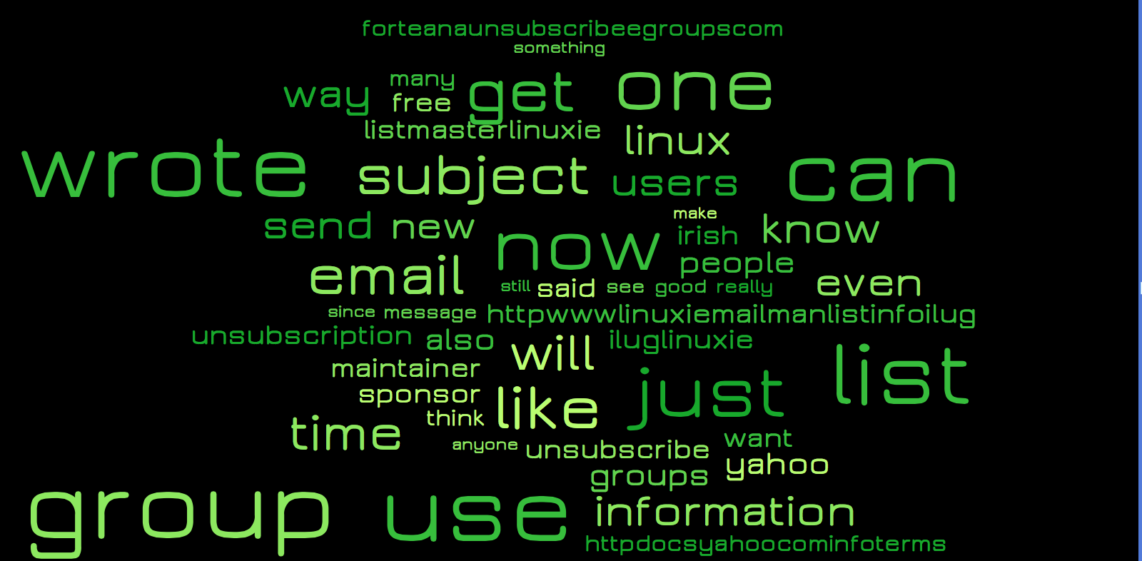
Given the tables, I've generated images using a wordcloud for some more insight. Let's take a look at the top 50 words for each table as represented in these images. Note that the red words are from the spam table and the green words are from the ham table. Additionally, the size of the words represents the occurrence rate. Thus the larger the word, the more documents contained that word at least once.

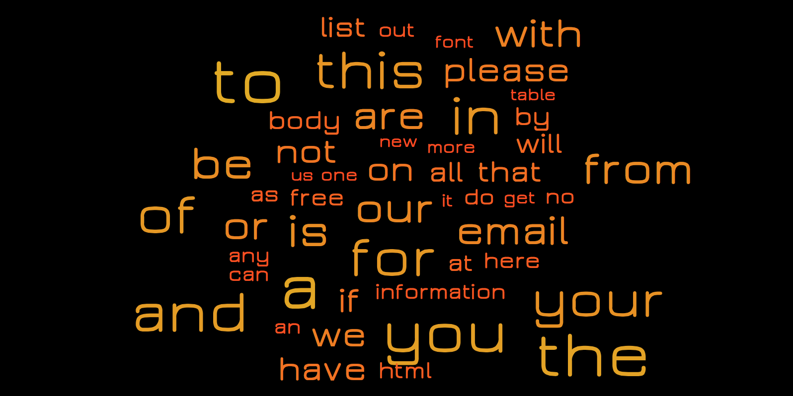
As you can see, mostly stop words come forward. These stop words are noise, which we should prevent as much as possible in our feature selection. Thus we should remove these from the tables before selecting the features. We've included a list of stop words in the example dataset. Let's first define the code to get these stop words.

  def getStopWords() : List[String] = { val source = scala.io.Source .fromFile(new File("/Users/.../.../Example Data/stopwords.txt"))("latin1") val lines = source.mkString.split("\n") source.close() return lines.toList } 

Now we can expand the TDM generation code with removing the stop words from the intermediate results:

val stopWords = getStopWords

val spamTDM  = spamMails .flatMap(email => email ._2.split(" ") .filter(word => word.nonEmpty && !stopWords.contains(word)) .map(word => (email._1.getName,word))) .groupBy(x => x._2) .map(x => (x._1, x._2.groupBy(x => x._1))) .map(x => (x._1, x._2.map( y => (y._1, y._2.length)))) .toList val hamTDM = hamMails .flatMap(email => email ._2.split(" ") .filter(word => word.nonEmpty && !stopWords.contains(word)) .map(word => (email._1.getName,word))) .groupBy(x => x._2) .map(x => (x._1, x._2.groupBy(x => x._1))) .map(x => (x._1, x._2.map( y => (y._1, y._2.length)))) .toList 

If we once again look at the top 50 words for spam and ham, we see that most of the stop words are gone. We could fine-tune more, but for now let's go with this.

With this insight in what 'spammy' words and what typical 'ham-words' are, we can decide on building a feature-set which we can then use in the Naive Bayes algorithm for creating the classifier. Note: it is always better to include more features, however performance might become an issue when having all words as features. This is why in the field, developers tend to drop features that do not have a significant impact, purely for performance reasons. Alternatively machine learning is done running complete Hadoop clusters, but explaining this would be outside the scope of this blog.

For now we will select the top 100 spammy words based on occurrence (thus not frequency) and do the same for ham words and combine this into 1 set of words which we can feed into the Bayes algorithm. Finally we also convert the training data to fit the input of the Bayes algorithm. Note that the final feature set thus is 200 - (#intersecting words *2). Feel free to experiment with higher and lower feature counts.

//Add the code for getting the TDM data and combining it into a feature bag.
val hamFeatures = hamTDM
    .records
    .take(amountOfFeaturesToTake)
    .map(x => x.term)

val spamFeatures = spamTDM .records .take(amountOfFeaturesToTake) .map(x => x.term) //Now we have a set of ham and spam features, // we group them and then remove the intersecting features, as these are noise. var data = (hamFeatures ++ spamFeatures).toSet hamFeatures .intersect(spamFeatures) .foreach(x => data = (data - x)) //Initialise a bag of words that takes the top x features //from both spam and ham and combines them var bag = new Bag[String] (data.toArray) //Initialise the classifier array with first a set of 0(spam) //and then a set of 1(ham) values that represent the emails var classifiers = Array.fill[Int](amountOfSamplesPerSet)(0) ++ Array.fill[Int](amountOfSamplesPerSet)(1) //Get the trainingData in the right format for the spam mails var spamData = spamMails .map(x => bag.feature(x._2.split(" "))) .toArray //Get the trainingData in the right format for the ham mails var hamData = hamMails .map(x => bag.feature(x._2.split(" "))) .toArray //Combine the training data from both categories var trainingData = spamData ++ hamData

Given this feature bag, and a set of training data, we can start training the algorithm. For this we can choose a few different models: General, Multinomial and Bernoulli. The General model needs to have a distribution defined, which we do not know on beforehand, so this is not a good option. The difference between the Multinomial and Bernoulli is the way in which they handle occurrence of words. The Bernoulli model only verifies whether a feature is there (binary 1 or 0), thus leaves out the statistical data of occurrences, where as the Multinomial model incorporates the occurrences (represented by the value). This causes the Bernoulli model to perform bad on longer documents in comparison to the Multinomial model. Since we will be rating emails, and we want to use the occurrence, we focus on the multinomial but feel free to try out the Bernoulli model as well.

//Create the bayes model as a multinomial with 2 classification
// groups and the amount of features passed in the constructor.

  var bayes = new NaiveBayes(NaiveBayes.Model.MULTINOMIAL, 2, data.size) //Now train the bayes instance with the training data, // which is represented in a specific format due to the //bag.feature method, and the known classifiers. bayes.learn(trainingData, classifiers)

Now that we have the trained model, we can once again do some validation. However, in the example data we already made a separation between easy and hard ham, and spam, thus we will not apply the cross validation, but rather validate the model using these test sets. We will start with validation of spam classification. For this we use the 1397 spam emails from the spam2 folder.

val listOfSpam2Files =   getFilesFromDir(spam2Path)
val spam2Mails = listOfSpam2Files .map{x => (x,getMessage(x)) } val spam2FeatureVectors = spam2Mails .map(x => bag.feature(x._2.split(" "))) val spam2ClassificationResults = spam2FeatureVectors .map(x => bayes.predict(x)) //Correct classifications are those who resulted in a spam classification (0) val correctClassifications = spam2ClassificationResults .count( x=> x == 0) println ( correctClassifications + " of " + listOfSpam2Files.length + "were correctly classified" ) println (( (correctClassifications.toDouble / listOfSpam2Files.length) * 100) + "% was correctly classified" ) //In case the algorithm could not decide which category the email //belongs to, it gives a -1 (unknown) rather than a 0 (spam) or 1 (ham) val unknownClassifications = spam2ClassificationResults .count( x=> x == -1) println( unknownClassifications + " of " + listOfSpam2Files.length + "were unknowingly classified" ) println( ( (unknownClassifications.toDouble / listOfSpam2Files.length) * 100) + % was unknowingly classified"  ) 

If we run this code several times with different feature amounts, we get the following results:

amountOfFeaturesToTake	Spam (Correct)	Unknown	Ham
50	1281 (91.70%)	16 (1.15%)	100 (7.15%)
100	1189 (85.11%)	18 (1.29%)	190 (13.6%)
200	1197 (85.68%)	16 (1.15%)	184 (13.17%)
400	1219 (87.26%)	13 (0.93%)	165 (11.81%)

Note that the amount of emails classified as Spam are the ones that are correctly classified by the model. Interestingly enough, the algorithm works best for classifying spam with only 50 features. However, recall that there were still stop words in the top 50 classification terms which could explain this result. If you look at how the values change as the amount of features increase (starting at 100), you can see that with more features, the overall result increases. Note that there is a group of unknown emails. For these emails the prior was equal for both classes. Note that this also is the case if there are no feature words for ham nor spam in the email, because then the algorithm would classify it 50% ham and 50% spam.

We will now do the same classification process for the ham emails. This is done by changing the path from the variablelistOfSpam2Files to easyHam2Path and rerunning the code. This gives us the following results:

amountOfFeaturesToTake	Spam	Unknown	Ham (Correct)
50	120 (8.57%)	28 ( 2.0%)	1252 (89.43%)
100	44 (3.14%)	11 (0.79%)	1345 (96.07%)
200	36 (2.57%)	7 (0.5%)	1357 (96.93%)
400	24 (1.71%)	7 (0.5%)	1369 (97.79%)

Note that now the correctly classified emails are those who are classified as ham. Here we see that indeed, when you use only 50 features, the amount of ham that gets classified correctly is significantly lower in comparison to the correct classifications when using 100 features. You should be aware of this and always verify your model for all classes, so in this case for both spam and ham test data.

To recap the example, we've worked through how you can use Naive Bayes to classify email as ham or spam, and got results of up to 87.26% correct classification for spam and 97.79% for ham. This shows that Naive Bayes indeed performs pretty well for classifying email as ham or spam.

With this we end the example of Naive Bayes. If you want to play around a bit more with Naive Bayes and Spam classification the corpus website also has a set of 'hard ham' emails that you could try to classify correctly by tweaking the feature amounts and removing more stopwords.

 Ranking emails based on their content (Recommendation system)

This example will be completely about building your own recommendation system. We will be ranking emails based on the following features: 'sender', 'subject', 'common terms in subject' and 'common terms in email body'. Later on in the example we will explain each of these features. Note that these features are for you to be defined when you make your own recommendation system. When building your own recommendation system this is one of the hardest parts. Coming up with good features is not trivial, and when you finally selected features the data might not be directly usable for these features.

The main idea behind this example is to show you how to do this feature selection, and how to solve issues that occur when you start doing this with your own data.

We will use a subset of the email data which we used in the example Classifying email as spam or ham. This subset can be downloaded here. Additionally you need the stop words file. Note that the data is a set of received emails, thus we lack half of the data, namely the outgoing emails of this mailbox. However even without this information we can do some pretty nice ranking as we will see later on.

Before we can do anything regarding the ranking system, we first need to extract as much data as we can from our email set. Since the data is a bit tedious in its format we provide the code to do this. The inline comments explain why things are done the way they are. Note that the application is a swing application with a GUI from the start. We do this because we will need to plot data in order to gain insight later on. Also note that we directly made a split in testing and training data such that we can later on test our model.

import java.awt.{Rectangle}
import java.io.File import java.text.SimpleDateFormat import java.util.Date import smile.plot.BarPlot import scala.swing.{MainFrame, SimpleSwingApplication} import scala.util.Try object RecommendationSystem extends SimpleSwingApplication { case class EmailData(emailDate : Date, sender : String, subject : String, body : String) def top = new MainFrame { title = "Recommendation System Example" val basePath = "/Users/../data" val easyHamPath = basePath + "/easy_ham" val mails = getFilesFromDir(easyHamPath).map(x => getFullEmail(x)) val timeSortedMails = mails .map (x => EmailData ( getDateFromEmail(x), getSenderFromEmail(x), getSubjectFromEmail(x), getMessageBodyFromEmail(x) ) ) .sortBy(x => x.emailDate) val (trainingData, testingData) = timeSortedMails .splitAt(timeSortedMails.length / 2) } def getFilesFromDir(path: String): List[File] = { val d = new File(path) if (d.exists && d.isDirectory) { //Remove the mac os basic storage file, //and alternatively for unix systems "cmds" d.listFiles.filter(x => x.isFile && !x.toString.contains(".DS_Store") && !x.toString.contains("cmds")).toList } else { List[File]() } } def getFullEmail(file: File): String = { //Note that the encoding of the example files is latin1, //thus this should be passed to the from file method. val source = scala.io.Source.fromFile(file)("latin1") val fullEmail = source.getLines mkString "\n" source.close() fullEmail } def getSubjectFromEmail(email: String): String = { //Find the index of the end of the subject line val subjectIndex = email.indexOf("Subject:") val endOfSubjectIndex = email .substring(subjectIndex) .indexOf('\n') + subjectIndex //Extract the subject: start of subject + 7 // (length of Subject:) until the end of the line. val subject = email .substring(subjectIndex + 8, endOfSubjectIndex) .trim .toLowerCase //Additionally, we check whether the email was a response and //remove the 're: ' tag, to make grouping on topic easier: subject.replace("re: ", "") } def getMessageBodyFromEmail(email: String): String = { val firstLineBreak = email.indexOf("\n\n") //Return the message body filtered by only text //from a-z and to lower case email.substring(firstLineBreak) .replace("\n", " ") .replaceAll("[^a-zA-Z ]", "") .toLowerCase } def getSenderFromEmail(email: String): String = { //Find the index of the From: line val fromLineIndex = email .indexOf("From:") val endOfLine = email .substring(fromLineIndex) .indexOf('\n') + fromLineIndex //Search for the <> tags in this line, as if they are there, // the email address is contained inside these tags val mailAddressStartIndex = email .substring(fromLineIndex, endOfLine) .indexOf('<') + fromLineIndex + 1 val mailAddressEndIndex = email .substring(fromLineIndex, endOfLine) .indexOf('>') + fromLineIndex if (mailAddressStartIndex > mailAddressEndIndex) { //The email address was not embedded in <> tags, // extract the substring without extra spacing and to lower case var emailString = email .substring(fromLineIndex + 5, endOfLine) .trim .toLowerCase //Remove a possible name embedded in () at the end of the line, //for example in test@test.com (tester) the name would be removed here val additionalNameStartIndex = emailString.indexOf('(') if (additionalNameStartIndex == -1) { emailString .toLowerCase }