Standard Deviation And Correlation

2019独角兽企业重金招聘Python工程师标准>>>

1: Introduction

In this mission, we'll be calculating statistics using data from the National Basketball Association (NBA). Here are the first few rows of thecsv file we'll be exploring:

"pts" is total points scored

"pf" column in the data is the total number of personal fouls each player had called on them in the season

"fta"(free throws attempted) 

"stl"(steals) 

FGM是 Field Goal Made 的缩写，意思是命中(次数)
FGA 是 Field Goal Attempted的缩写，意思是投射(次数)，或者说是出手次数。

 

G：（games）出场比赛
GS：（games started）首发比赛
MP：（minutes played）比赛时间（分钟）
FG：（field goals）投中球
FT：（free throws）罚球命中次数
AST：（assists） 助攻次数
STL：（steals ） 抢断次数
BLK：（blocks）盖帽次数
TOV： （turnovers）失误次数
PF：（personal fouls）犯规次数
PTF：（points）球员得分

 

 

player,pos,age,bref_team_id,g,gs,mp,fg,fga,fg.,x3p,x3pa,x3p.,x2p,x2pa,x2p.,efg.,ft,fta,ft.,orb,drb,trb,ast,stl,blk,tov,pf,pts,season

    ,season_end

Quincy Acy,SF,23,TOT,63,0,847,66,141,0.468,4,15,0.266666666666667,62,126,0.492063492063492,0.482,35,53,0.66,72,144,216,28,23,26,30,122

    ,171,2013-2014,2013

Steven Adams,C,20,OKC,81,20,1197,93,185,0.503,0,0,NA,93,185,0.502702702702703,0.503,79,136,0.581,142,190,332,43,40,57,71,203,265,2013

    -2014,2013

Each row contains data on a single player for a single season. It contains statistics such as the team the player played on, how many points they scored in the season, and more.

Here are some of the interesting columns:

• player -- name of the player.
• pts -- the total number of points the player scored in the season.
• ast -- the total number of assists the player had in the season.
• fg. -- the player's field goal percentage for the season.

In the next few screens, we'll dive into this dataset and calculate some summary statistics that help us explore the data.

2: The Mean As The Center

We have looked briefly at the mean before, but it has an interesting property.

If we subtract the mean of a set of numbers from each of the numbers, the differences will always add up to zero.

This is because the mean is the "center" of the data. All of the differences that are negative will always cancel out all of the differences that are positive.

Let's look at some examples to verify this.

Let's also get familiar with the mathematical symbol for the mean -- x¯x¯ -- this symbol means "the average of all the values in x". The fact that x is lowercase but bold means that it is a vector. The bar over the top means "the average of".

Instructions

• Find the median of the valueslist. Assign the result tovalues_median.

• Subtract the median from each element in values. Sum up all of the differences, and assign the result tomedian_difference_sum

# Make a list of values
values = [2, 4, 5, -1, 0, 10, 8, 9]
# Compute the mean of the values
values_mean = sum(values) / len(values)
# Find the difference between each of the values and the mean by subtracting the mean from each value.
differences = [i - values_mean for i in values]
# This equals 0.  Try changing the values around and verifying that it equals 0 if you want.
print(sum(differences))

# We can use the median function from numpy to find the median
# The median is the "middle" value in a set of values -- if you sort the values in order, it's the one in the center (or the average of the two in the center if there are an even number of items in the set)
# You'll see that the differences from the median don't always add to 0.  You might want to play around with this and think about why that is.
from numpy import median
values_median=median(values)
differences=[i-values_median for i in values]
median_difference_sum=sum(differences)

 

3: Finding Variance

Let's look at variance in the data.

Variance tells us how "spread out" the data is around the mean.

We looked at kurtosis earlier, which measures the shape of a distribution.

Variance directly measures how far from the mean the average element in the data is.

We calculate variance by subtracting every value from the mean, squaring the results, and averaging them.

Mathemically, this looks like σ2=∑i=1n(xi−x¯)2nσ2=∑i=1n(xi−x¯)2n. σ2σ2 is variance, ∑ni=1∑i=1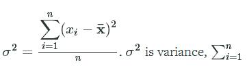n means "the sum from 1 to n", where n is the number of elements in a vector. The formula does the exact same thing we just described, but is the most common way to show it.

The "pf" column in the data is the total number of personal fouls each player had called on them in the season -- let's look at its variance.

Instructions

• Compute the variance of the"pts" column in the data --"pts" is total points scored.

• Assign the result topoint_variance.import matplotlib.pyplot as plt
  import pandas as pd
  # The nba data is loaded into the nba_stats variable.
  # Find the mean value of the column
  pf_mean = nba_stats["pf"].mean()
  # Initialize variance at zero
  variance = 0
  # Loop through each item in the "pf" column
  for p in nba_stats["pf"]:
      # Calculate the difference between the mean and the value
      difference = p - pf_mean
      # Square the difference -- this ensures that the result isn't negative
      # If we didn't square the difference, the total variance would be zero
      # ** in python means "raise whatever comes before this to the power of whatever number is after this"
      square_difference = difference ** 2
      # Add the difference to the total
      variance += square_difference
  # Average the total to find the final variance.
  variance = variance / len(nba_stats["pf"])
  pts_mean=nba_stats["pts"].mean()
  point_variance =0
  for p in nba_stats["pts"]:
      difference=p-pts_mean
      square_difference=difference**2
      point_variance +=square_difference
      
  point_variance= point_variance /len(nba_stats["pts"])

•  

   

   

   

  4: Order Of Operations

  We've been multiplying and dividing values, but we haven't really discussed order of operations yet.

  Order of operations define which mathematical operations occur in which sequence.

  Think about 2 * 5 - 1 -- depending on whether we do the multiplication first, or the subtraction first, the result will change.

  If we multiply first, we get 10 - 1, which equals 9.

  If we subtract first, we get 2 * 4, which equals 8.

  We definitely want the results of these operations to be consistent -- we don't want to sometimes get 8, and sometimes get 9.

  Because of this, we have an order of operations.

  At the top is raising something to a power (x ** y), then multiplication (x * y) and division (x / y) are equal, and then addition (x + y) and subtraction (x - y) are equal.

  So raising something to a power will always happen first, then any multiplication/division, and last any addition/subtraction.

  We'll play around with this to get a better feel for it.

  Instructions

• Change the mathematical operations around so that cequals 25, and d equals .5.

 

# You might be wondering why multiplication and division are on the same level.
# It doesn't matter whether we do the multiplication first, or the division first -- the answer here will always be the same.
# In this case, we need to think of division as multiplication by a fraction -- otherwise, we'll be dividing more than we want to.
# Create a formula
a = 5 * 5 / 2
# Multiply by 1/2 instead of dividing by 2 -- the result is the same (2/2 == 2 * 1/2)
a_subbed = 5 * 5 * 1/2
a_mul_first = 25 * 1/2
a_div_first = 5 * 2.5
print(a_mul_first == a_div_first)

# The same thing is true for subtraction and addition
# In this case, we need to convert subtraction into adding a negative number -- if we don't we'll end up subtracting more than we expect
b = 10 - 8 + 5
# Add -8 instead of subtracting 8
b_subbed = 10 + -8 + 5
b_sub_first = 2 + 5
b_add_first = 10 + -3
print(b_sub_first == b_add_first)

c = 10 / 2 * 5
d = 3 - 1 / 2 -2

 

 

5: Using Parentheses

Parentheses can be used to "override" the order of operations and make something happen first.

For example 10 - 2 / 2 will equal 9, because the division happens before the subtraction.

If we write (10 - 2) / 2, the parentheses "force" the part inside to happen first, so we end up with 8/2.

Instructions

• Use parentheses to make b equal1100.

• Use parentheses to make c equal200.

a = 50 * 50 - 10 / 5
a_paren = 50 * (50 - 10) / 5
# If we put multiple operations inside parentheses, the order of operations is used inside to determine the order.
a_paren = 50 * (50 - 10 / 5)

b = 10 * (10+ 100)
c =(8 - 6) * 100

 

6: Fractional Powers

Before we explore variance a little more, let's take a quick look at exponents.

We did difference ** 2 in the last screen, which squared the difference -- this is equal to difference * difference.

We could cube the difference by doing difference ** 3 -- this is equal to difference * difference * difference.

This same pattern holds true as we raise to higher powers, like 4, 5, and so on.

We can also take roots of numbers with the same syntax.

difference ** (1/2) will take the square root -- we need to put the fraction in parentheses because raising a value to a power always happens first normally.

difference ** (1/3) will take the cube root. And so on with smaller fractions.

Instructions

• Raise 11 to the fifth power. Assign the result to e.

• Take the fourth root of 10000. Assign the result to f

a = 5 ** 2
# Raise to the fourth power
b = 10 ** 4

# Take the square root ( 3 * 3 == 9, so the answer is 3)
c = 9 ** (1/2)

# Take the cube root (4 * 4 * 4 == 64, so 4 is the cube root)
d = 64 ** (1/3)
e=11**(5)
f=10000**(1/4)

 

7: Calculating Standard Deviation

A commonly used way to refer to how far data points are from the mean is called standard deviation.

It is typical to measure what percentage of the data is within 1 standard deviation of the mean, or two standard deviations of the mean.

Standard deviation is a very useful concept, and is a great way to measure how spread out data is.

Luckily for us, standard deviation is just the square root of the variance.

Here's the mathematical formula for standard deviation -- σ=∑i=1n(xi−x¯)2n−−−−−−−−−−−⎷σ=∑i=1n(xi−x¯)2n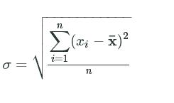

Instructions

 

 

 

• Make a function that calculates the standard deviation of a given column in the nba_stats data.

• Use the function to calculate the standard deviation for the minutes played column ("mp"). Assign the results to mp_dev.

• Use the function to calculate the standard deviation for the assists column ("ast"). Assign the results to ast_dev

# The nba stats are loaded into the nba_stats variable.
mean_mp_dev=nba_stats["mp"].mean()
mp_variance=0
for p_mp in nba_stats["mp"]:
    difference=p_mp-mean_mp_dev
    square_difference=difference**2
    mp_variance+=square_difference
    
mp_dev=(mp_variance/len(nba_stats["mp"]))**(1/2)

mean_ast_dev=nba_stats["ast"].mean()
ast_variance=0
for p_ast in nba_stats["ast"]:
    difference=p_ast-mean_ast_dev
    square_difference=difference**2
    ast_variance+=square_difference
    
ast_dev=(ast_variance/len(nba_stats["ast"]))**(1/2)

    
    

8: Find Standard Deviation Distance

The standard deviation is very useful because it lets us compare points in a distribution to the mean.

We can say that a certain point is "two standard deviations away from the mean".

This gives us a way to compare how spread out values are across different charts.

Instructions

• Find how many standard deviations away from the meanpoint_10 is. Assign the result topoint_10_std.

• Find how many standard deviations away from the meanpoint_100 is. Assign the result to point_100_std.

import matplotlib.pyplot as plt

plt.hist(nba_stats["pf"])
mean = nba_stats["pf"].mean()
plt.axvline(mean, color="r")
# We can calculate standard deviation by using the std() method on a pandas series.
std_dev = nba_stats["pf"].std()
# Plot a line one standard deviation below the mean
plt.axvline(mean - std_dev, color="g")
# Plot a line one standard deviation above the mean
plt.axvline(mean + std_dev, color="g")

# We can see how much of the data points fall within 1 standard deviation of the mean
# The more that falls into this range, the less spread out the data is
plt.show()

# We can calculate how many standard deviations a data point is from the mean by doing some subtraction and division
# First, we find the total distance by subtracting the mean
total_distance = nba_stats["pf"][0] - mean
# Then we divide by standard deviation to find how many standard deviations away the point is.
standard_deviation_distance = total_distance / std_dev

point_10 = nba_stats["pf"][9]
point_100 = nba_stats["pf"][99]
point_10_std=(point_10-mean)/std_dev
point_100_std=(point_100-mean)/std_dev

9: Working With The Normal Distribution

The normal distribution is a special kind of distribution.

You might recognize it more commonly as a bell curve.

The normal distribution is found in a variety of natural phenomena. For example, if you made a histogram of the heights of all humans, it would be more or less a normal distribution.

We can generate a normal distribution by using a probability density function.

Instructions

 

 

• Make a normal distribution across the range that starts at-10, ends at 10, and has the step.1.

• The distribution should have mean 0 and standard deviation of 2

import numpy as np
import matplotlib.pyplot as plt
# The norm module has a pdf function (pdf stands for probability density function)
from scipy.stats import norm

# The arange function generates a numpy vector
# The vector below will start at -1, and go up to, but not including 1
# It will proceed in "steps" of .01.  So the first element will be -1, the second -.99, the third -.98, all the way up to .99.
points = np.arange(-1, 1, 0.01)

# The norm.pdf function will take points vector and turn it into a probability vector
# Each element in the vector will correspond to the normal distribution (earlier elements and later element smaller, peak in the center)
# The distribution will be centered on 0, and will have a standard devation of .3
probabilities = norm.pdf(points, 0, .3)

# Plot the points values on the x axis and the corresponding probabilities on the y axis
# See the bell curve?
plt.plot(points, probabilities)
plt.show()
points=np.arrange(-10,10,0.1)
probabilities=norm.pdf(points,0,2)
plt.plot(points,probabilities)
plt.show()

 

import numpy as np
import matplotlib.pyplot as plt
# The norm module has a pdf function (pdf stands for probability density function)
from scipy.stats import norm

# The arange function generates a numpy vector
# The vector below will start at -1, and go up to, but not including 1
# It will proceed in "steps" of .01.  So the first element will be -1, the second -.99, the third -.98, all the way up to .99.
points = np.arange(-1, 1, 0.01)

# The norm.pdf function will take points vector and turn it into a probability vector
# Each element in the vector will correspond to the normal distribution (earlier elements and later element smaller, peak in the center)
# The distribution will be centered on 0, and will have a standard devation of .3
probabilities = norm.pdf(points, 0, .3)

# Plot the points values on the x axis and the corresponding probabilities on the y axis
# See the bell curve?
plt.plot(points, probabilities)
plt.show()
points=np.arrange(-10,10,0.1)
probabilities=norm.pdf(points,0,2)
plt.plot(points,probabilities)
plt.show()

 

10: Normal Distribution Deviation

One cool thing about normal distributions is that for every single one, the same percentage of the data is within 1 standard deviation of the mean, the same percentage is within 2 standard deviations of the mean, and so on.

About 68% of the data is within 1 standard deviation of the mean, about 95% is within 2 standard deviations of the mean, and about 99% is within 3 standard deviations of the mean.

This helps us to quickly understand where values fall and how unusual they are.

Instructions

• For each point in wing_lengths, calculate the number of standard deviations away from the mean the point is.

• Compute what percentage of the data is within 1 standard deviation of the mean. Assign the result towithin_one_percentage.

• Compute what percentage of the data is within 2 standard deviations of the mean. Assign the result towithin_two_percentage.

• Compute what percentage of the data is within 3 standard deviations of the mean. Assign the result towithin_three_percentage

# Housefly wing lengths in millimeters
 

# Housefly wing lengths in millimeters
wing_lengths = [36, 37, 38, 38, 39, 39, 40, 40, 40, 40, 41, 41, 41, 41, 41, 41, 42, 42, 42, 42, 42, 42, 42, 43, 43, 43, 43, 43, 43, 43, 43, 44, 44, 44, 44, 44, 44, 44, 44, 44, 45, 45, 45, 45, 45, 45, 45, 45, 45, 45, 46, 46, 46, 46, 46, 46, 46, 46, 46, 46, 47, 47, 47, 47, 47, 47, 47, 47, 47, 48, 48, 48, 48, 48, 48, 48, 48, 49, 49, 49, 49, 49, 49, 49, 50, 50, 50, 50, 50, 50, 51, 51, 51, 51, 52, 52, 53, 53, 54, 55]
mean = sum(wing_lengths) / len(wing_lengths)
variances = [(i - mean) ** 2 for i in wing_lengths]
variance = sum(variances)/ len(variances)
standard_deviation = variance ** (1/2)

standard_deviations = [(i - mean) / standard_deviation for i in wing_lengths]
def within_percentage(deviations, count):
    within = [i for i in deviations if i <= count and i >= -count]
    count = len(within)
    return count / len(deviations)

within_one_percentage = within_percentage(standard_deviations, 1)
within_two_percentage = within_percentage(standard_deviations, 2)
within_three_percentage = within_percentage(standard_deviations, 3)

 

 

11: Plotting Correlations

We've spent a lot of time looking at single variables and how their distributions look.

While distributions are interesting on their own, it's also interesting to look at how two variables correlate with each other.

A lot of statistics is about analyzing how variables impact each other, and the first step is to graph them out with a scatterplot.

While graphing them out, we can look at correlation.

If two variables both change together (ie, when one goes up, the other goes up), we know that they are correlated.

Instructions

• Make a scatterplot of the "fta"(free throws attempted) column against the "pts" column.

• Make a scatterplot of the "stl"(steals) column against the "pf"column.

import matplotlib.pyplot as plt
# This is plotting field goals attempted (number of shots someone takes in a season) vs point scored in a season
# Field goals attempted is on the x-axis, and points is on the y-axis
# As you can tell, they are very strongly correlated -- the plot is close to a straight line.
# The plot also slopes upward, which means that as field goal attempts go up, so do points.
# That means that the plot is positively correlated.
plt.scatter(nba_stats["fga"], nba_stats["pts"])
plt.show()
# If we make points negative (so the people who scored the most points now score the least, because 3000 becomes -3000), we can change the direction of the correlation
# Field goals are negatively correlated with our new "negative" points column -- the more free throws you attempt, the less negative points you score.
# We can see this because the correlation line slopes downward.
plt.scatter(nba_stats["fga"], -nba_stats["pts"])
plt.show()
# Now, we can plot total rebounds (number of times someone got the ball back for their team after someone shot) vs total assists (number of times someone helped another person score)
# These are uncorrelated, so you don't see the same nice line as you see with the plot above.
plt.scatter(nba_stats["trb"], nba_stats["ast"])
plt.show()
plt.scatter(nba_stats["fta"],nba_stats["pts"])
plt.show()
plt.scatter(nba_stats["stl"],nba_stats["pf"])
plt.show()

12: Measuring Correlation

One thing that can help us a lot when we need to analyze a lot of variables is to measure correlation -- this means that we don't need to eyeball everything.

The most common way to measure correlation is to use Pearson's r, also called an r-value.

We'll go through how the calculations work, but for now, we'll focus on the values.

An r-value ranges from -1 to 1, and indicates how strongly two variables are correlated.

A 1 means perfect positive correlation -- this would show as a straight, upward-sloping line on our plots.

A 0 means no correlation -- you'll see a scatterplot with points placed randomly.

A -1 means perfect negative correlation -- this would show as a straight, downward-sloping line.

Anything between -1 and 0, and 0 and 1 will show up as a scattering of points. The closer the value is to 0, the more random the points will look. The closer to -1 or 1, the more like a line the points will look.

We can use a function from scipy to calculate Pearson's r for the moment.

Instructions

• Find the correlation between the"fta" column and the "pts"column. Assign the result tor_fta_pts.

• Find the correlation between the"stl" column and the "pf"column. Assign the result tor_stl_pf.

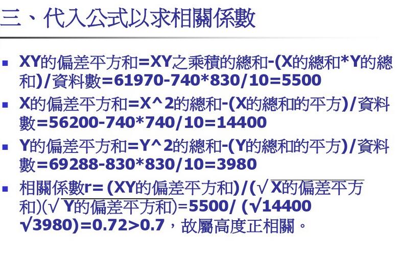
（原理）

• 

 

from scipy.stats.stats import pearsonr

# The pearsonr function will find the correlation between two columns of data.
# It returns the r value and the p value.  We'll learn more about p values later on.
r, p_value = pearsonr(nba_stats["fga"], nba_stats["pts"])
# As we can see, this is a very high positive r value -- close to 1
print(r)

# These two columns are much less correlated
r, p_value = pearsonr(nba_stats["trb"], nba_stats["ast"])
# We get a much lower, but still positive, r value
print(r)

r_fta_pts, p_value = pearsonr(nba_stats["fta"], nba_stats["pts"])

r_stl_pf, p_value = pearsonr(nba_stats["stl"], nba_stats["pf"])

 

13: Calculate Covariance

We looked at calculating the correlation coefficient with a function, but let's briefly look under the hood to see how we can do it ourselves.

Another way to think of correlation is in terms of variance.

Two variables are correlated when they both individually vary in similar ways.

For example, correlation occurs when if one variable goes up, another variable also goes up.

This is called covariance. Covariance is how things vary together.

There is a maximum amount of how much two variables can co-vary.

This is because of how each variable is individually distributed. Each individual distribution has its own variance. These variances set a maximum theoretical limit on covariance between two variables -- you can't co-vary more from the mean than the two variables individually vary from the mean.

The r-value is a ratio between the actual covariance, and the maximum possible positive covariance.

The maximum possible covariance occurs when two variables vary perfectly (ie, you see a straight line on the plot).

Let's look at actual covariance first. Mathematically speaking, covariance between two variables looks like this: cov(x,y)=∑ni=1(xi−x¯)(yi−y¯)ncov(x,y)=∑i=1n(xi−x¯)(yi−y¯)n.

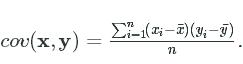
For each element in the vectors x and y, you take the value at each position from 1 to the length of the vectors. Subtract the mean of the vector from that value. Then multiply them together at each position, and all of the resulting values together.

Instructions

• Make a function to compute covariance.

• Use the function to compute the covariance of the "stl" and"pf" columns. Assign the result to cov_stl_pf.

• Use the function to compute the covariance of the "fta" and"pts" columns. Assign the result to cov_fta_pts.

巧妙地函数应用

# The nba_stats variable has been loaded.
def covariance(x,y):
    x_mean=sum(x)/len(x)
    y_mean=sum(y)/len(y)
    x_diffs=[i-x_mean for i in x]
    y_diffs=[i-y_mean for i in y]
    codeviates=[x_diffs[i]*y_diffs[i] for i in range(len(y))]
    return sum(codeviates)/len(codeviates)
    
cov_stl_pf=covariance(nba_stats["stl"],nba_stats["pf"])
cov_fta_pts=covariance(nba_stats["fta"],nba_stats["pts"])

 

 

 

14: Calculate Correlation

Now that we know how to calculate covariance, we can calculate the correlation coefficient using the following formula:

cov(x,y)σxσycov(x,y)σxσy.

For the denominator, we need to multiple the standard deviations for x and y. This is the maximum possible positive covariance -- it's just both the standard deviation values multiplied. If we divide our actual covariance by this, we get the r-value.

You can use the std method on any Pandas Dataframe or Series to calculate the standard deviation. The following code returns the standard deviation for the pf column:

 

nba_stats["pf"].std()

You can use the cov function from NumPy to compute covariance, returning a 2x2 matrix. The following code returns the covariance between the pf and stl columns:

 

cov(nba_stats["pf"], nba_stats["stl"])[0,1]

Instructions

• Compute the correlation coefficient for the fta and blkcolumns and assign the result tor_fta_blk.

• Compute the correlation coefficient for the ast and stlcolumns and assign the result tor_ast_stl.

from numpy import cov
# The nba_stats variable has already been loaded.
r_fta_blk=cov(nba_stats["fta"], nba_stats["blk"])[0,1]/((nba_stats["fta"].var()*nba_stats["blk"].var())**(1/2))
r_ast_stl=cov(nba_stats["ast"], nba_stats["stl"])[0,1]/((nba_stats["ast"].var()*nba_stats["stl"].var())**(1/2))

 

 

转载于:https://my.oschina.net/Bettyty/blog/748268